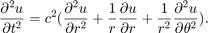
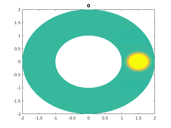
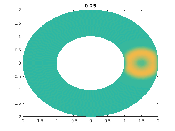
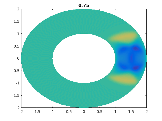
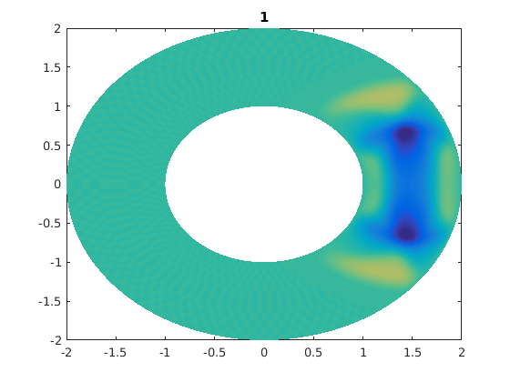
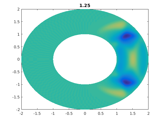
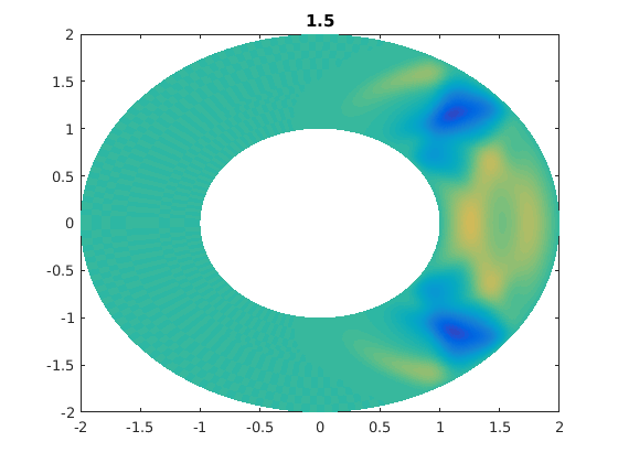
Wave Equation on an Annular Domain

This code solves a wave equation on an annular domain. Please note that this script defines functions at the end, which is only supported by MATLAB 2016b or later. The method is Chebyshev pseudospectral in r. The method is matrix based Fourier in theta. In polar coordinates the equation is written as:

$\frac{\partial^2 u}{\partial t^2} = c^2 (\frac{\partial^2 u}{\partial r^2} + \frac{1}{r} \frac{\partial u}{\partial r} + \frac{1}{r^2} \frac{\partial^2 u}{\partial\theta^2}).$

Initialization
Chebyshev function

clear, close all;

Initialization

Grid sizes.

Nx=96*2;
Ny=64;

Chebyshev in yc (the computational coordinate in the radial direction).

[Dyc,yc]=cheb(Ny);

Fourier in xc (the computational coordinate for theta).

dxc = 2*pi/Nx;
xc = -pi + (1:Nx)'*dxc;
column = [0 .5*(-1).^(1:Nx-1).*cot((1:Nx-1)*dxc/2)];
Dxc = toeplitz(column,column([1 Nx:-1:2]));

Physical domain parameters and scaling for the physical grid.

Rin=1; % Inner radius.
Rout=2; % Outer radius.
dR=Rout-Rin; % Difference in radii.
theta=xc;
Dtheta=Dxc;
r=Rin+(yc+1)*0.5*dR;
[rr,thth]=meshgrid(r,theta);

For the operator on RHS.

over=1./r;
Dr=Dyc*(2/dR);
overr=1./rr;
overrr2=(1./rr).^2;
Dthetatheta=Dtheta*Dtheta; Drr=Dr*Dr;

Definitions for the Cartesian coordinates.

xx=rr.*cos(thth);
yy=rr.*sin(thth);

Initial conditions.

un=sech(((xx-1.5).^2+yy.^2)/0.25).^16;
up=un;

Parameters for plotting.

Ngx=1000;
Ngy=200;
rg=linspace(Rin,Rout,Ngy+1);
thg=linspace(-pi,pi,Ngx+1);
[rrg,ththg]=meshgrid(rg,thg);
xxg=rrg.*cos(ththg);
yyg=rrg.*sin(ththg);

Time stepping parameters.

% numsteps=20; numouts=500; dt=0.001; dt2=dt*dt; c=1; c2=c*c;
% The above is the version for "live" movies.
numsteps=250;
numouts=9;
dt=0.001;
dt2=dt*dt;
c=1;
c2=c*c;
t=0;
for ii=1:numouts

    ung=interp2(rr,thth,un,rrg,ththg,'spline');
    % I use spline because it can handle the extrapolation as well.
    % I also make sure the grid wraps around so as to show the whole
    % annular domain.

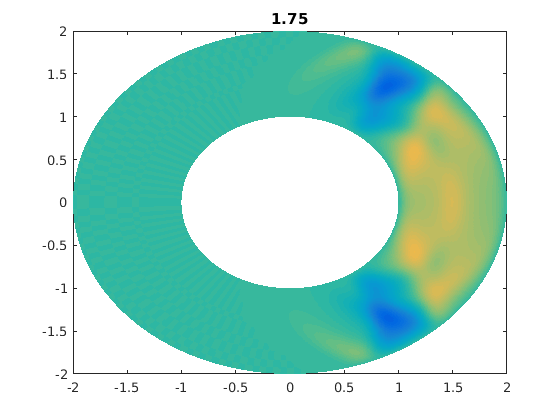
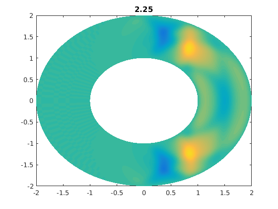
    %figure(ii) % For publishable version.
    figure(1) % For live movies.
    clf
    pcolor(xxg,yyg,ung),shading flat,caxis([-1 1]*0.5)
    % I caxis with a smaller range of values.
    % I do this so that later times are clearer.
    title(t)
    drawnow

    for jj=1:numsteps

        t=t+dt;

        rhs=un*Drr'+overr.*(un*Dr')+overrr2.*(Dthetatheta*un);
        % Notice I can use fairly reasonably sized matrices.
        % This is because I keep the u variable as a matrix.
        % This means I need to get my left vs right multiplications
        % correct.
        uf=2*un-up+dt2*c2*rhs;
        uf(:,1)=0;
        uf(:,end)=0;
        up=un;
        un=uf;

end

end

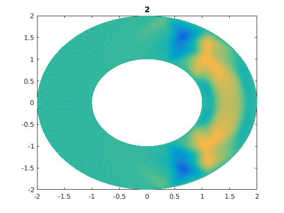
And one last picture.

%figure(numouts+1)
figure(2)
clf
ung=interp2(rr,thth,un,rrg,ththg,'spline');
pcolor(xxg,yyg,ung),shading flat,caxis([-1 1]*0.5)
title(t),drawnow

Chebyshev function

CHEB compute D = differentiation matrix, x = Chebyshev grid

function [D,x] = cheb(N)
if N==0, D=0; x=1; return, end
x = cos(pi*(0:N)/N)';
c = [2; ones(N-1,1); 2].*(-1).^(0:N)';
X = repmat(x,1,N+1);
dX = X-X';
D  = (c*(1./c)')./(dX+(eye(N+1)));      % off-diagonal entries
D  = D - diag(sum(D'));                 % diagonal entries
end

Wave Equation on an Annular Domain

Contents

Initialization

Chebyshev function