SPINS Tutorial

This is a tutorial for getting up to speed with SPINS using the case mode1_mode2. You must first have followed the instructions to install SPINS and compile the case file.

Run

Transfer the executable (mode1_mode2.x) and the configuration file (spins.conf) into a clean directory.

Run simulation by executing mpirun -np 4 ./mode1_mode2.x on the command line, or submit the job to the queue on a Compute Canada system with a submit script (see submitting jobs to Graham).

This will create two types of files

1. Output files
   • These are of the form rho.3 where the name (rho) is the variable and the extension is the output number

   - For example rho.3 is the density field at output number 3. Zero-indexing is used, so this is the 4th density file

   • Since these can be memory expensive, they are created relatively infrequently
2. Diagnostic files
   • These will generally be text files and contain information about the simulation

Diagnostic Files
File	Optional	Matlab plotter	Description
diagnostics.txt	No	plot_diagnos	High temporal resolution information about the simulation (occurs at every time step). Examples include: KE, max velocity, energy budget terms, simulation timings.
stresses.txt (or stresses_top.txt and/or stresses_bottom.txt)	Yes	plot_stress	Surface forces (yes, it's a misnomer and needs to be fixed) at the top/bottom surfaces. Only useful if no slip boundary condition is used. Multiple integrals along the surfaces are completed.
plot_times.txt	No	plot_diagnos	Explicit statement of the time associated with each output. Also gives the time to write output files.

Analyze

Matlab and Python are the primary languages used for analyzing SPINS simulations. These are great for computation of quantities specific to your study. The Python (SPINSpy) and Matlab (SPINSmatlab) packages contain much of the important tools for each language. Three dimensional visualization should use Paraview or VisIt (see Visualization).

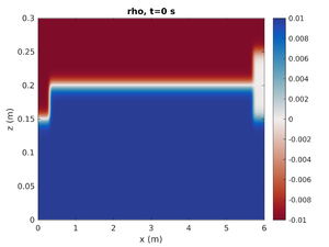
Here, we will use Matlab to make a simple plot of the density field. We assume that the SPINSmatlab package is on your path (as is the case for boogaloo).

1. gdpar = spins_gridparams(); split_gdpar
   • This reads in the grid and parameters and places them in a structure (gdpar). split_gdpar separates the two sub-structures into the structures par and gd, which are the parameters and grid, respectively.
   • par contains information from spins.conf in addition to further simulation parameters
   • gd contains the grid. x,y,z grids can be extracted with gd.x, gd.y, or gd.z
   • The default setting is that the grid is unmapped and vector grids are produced, to get the full grid use gdpar = spins_gridparams('FastFull'); or gdpar = spins_gridparams('Full');
2. spins_plot2d('rho',0);
   • First argument is the field to plot
   • Second argument is the output number. The simulation time can also be specified in this argument as a string. spins_plot2d('rho','2'); will plot the simulation at the closest output to t=2s. Many optional arguments exist (type help spins_plot2d for more options).

To read an individual file: u = spins_reader('u',10)

Restart

Should you need to restart the simulation (due to expenditure of allocated time, require more time, a node failure, or otherwise) simply change the restart flags in the configuration file.

The simplest change is to set

restart = true
restart_time = 5.5
restart_sequence = 11

where the simulation will restart at output 11 which corresponds to t=5.5s. These numbers can be found as the last row in plot_time.txt.

SPINS also has an automatic safety dump if the allocated time is close to expiring (See automatically specify the runtime for more info). In this case, if the safety write was done successfully then you only need to set

restart_from_dump = true

Change

If after analyzing the simulation you realize that you wanted to change a parameter (it wasn't quite right), then you only need to change the parameter in the configuration file (as opposed to older editions of SPINS where you'd need to recompile the entire code).

Here is a description of the problem parameters:

 --delta_rho     arg   Density difference between upper and lower layers (as a percentage of rho_0)
 --pyc_loc       arg   Pycnocline location
 --h_halfwidth   arg   Pycnocline half-width
 --delta_x       arg   Horizontal transition half-width
 --H2            arg   Height of mixed region (mode-2) - sets mode-2 wave amplitude
 --H1            arg   Heigth of mixed region (mode-1) - sets mode-1 wave amplitude
 --L1            arg   Length of region 1 (mode-2)
 --L2            arg   Length of region 2 (mode-1)
 --dye1_loc      arg   Location of dye 1
 --dye2_loc      arg   Location of dye 2
 --dye1_width    arg   Width of dye 1
 --dye2_width    arg   Width of dye 2
 --dye_halfwidth arg   Sharpness of the dye transition
 --enable_tracer       Enable evolution of second tracers

If you run the simulation in the same directory, remember to clear all simulation files (output and diagnostic files).

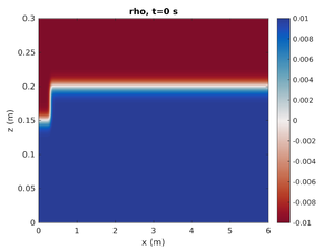
Only Mode-1 ISW

To change the simulation to only have the left mode-1 ISW change spins.conf to have:

H2 = 0.0

This will set the mode-2 amplitude to zero.

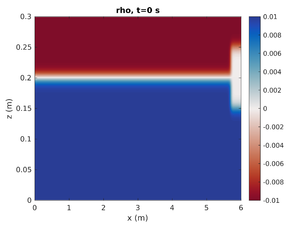
Only Mode-2 ISW

To change the simulation to only have the right mode-2 ISW change spins.conf to have:

H1 = 0.0

This will set the mode-1 amplitude to zero.

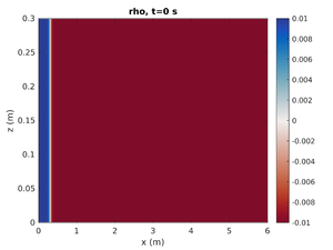
Gravity Current

To change the simulation to have a rightward moving gravity current change spins.conf to have:

pyc_loc = -0.2
H1 = -1.0
H2 = 0.0

This will move the pycnocline below the bottom boundary, set the mode-1 amplitude to result in a region of high density at on end of the tank, and give no mode-2 contribution.

Try it yourself. See what each parameter does when they're changed.