Gravity wave tutorial: Difference between revisions
No edit summary |
m (Fix old link to belize so it refers to this new wiki.) |
||
| (26 intermediate revisions by 2 users not shown) | |||
| Line 1: | Line 1: | ||
This tutorial is useful if you have never worked with the model before and want to very quickly get a sense of the main parts and offers a "hands on" alternative to sifting through the manual. The tutorial will also attempt to walk you through troubleshooting skills that will be useful as the manual becomes less so. For best results, do attempt the activities before looking at the walkthrough, and take note of references to the MITgcm user manual. Enjoy! | |||
This tutorial assumed you have followed the instructions for [[MITgcmSetup|setting up the model]] and for [[MITgcm_Tutorials|cloning the tutorial code]]. | |||
== Troubleshooting Resources == | == Troubleshooting Resources == | ||
The MITgcm Online Manual can be found [http://mitgcm.org/public/r2_manual/latest/ here]. A more useful, complete PDF file of the manual can be found [http://mitgcm.org/public/r2_manual/latest/online_documents/manual.pdf here]. The MITgcm help support mailing list can be found [http://mitgcm.org/mailman/listinfo/mitgcm-support here], and it is often useful to search the help inquiries (google with the addition site: mitgcm.org) if you are having a specific issue. Finally, the MITgcm is supported by a [http://mitgcm.org/public/r2_manual/latest/code_reference/callTree.html code browser] that allows you to track certain variables within the entire code base. Keep in mind that this search model may contain out-of-date code, but it is a useful resource for sourcing where problems may be found. The best option is always to track it down in your local version of the MITgcm! | The MITgcm Online Manual can be found [http://mitgcm.org/public/r2_manual/latest/ here]. A more useful, complete PDF file of the manual can be found [http://mitgcm.org/public/r2_manual/latest/online_documents/manual.pdf here]. The MITgcm help support mailing list can be found [http://mitgcm.org/mailman/listinfo/mitgcm-support here], and it is often useful to search the help inquiries (google with the addition site: mitgcm.org) if you are having a specific issue. Finally, the MITgcm is supported by a [http://mitgcm.org/public/r2_manual/latest/code_reference/callTree.html code browser] that allows you to track certain variables within the entire code base. Keep in mind that this search model may contain out-of-date code, but it is a useful resource for sourcing where problems may be found. The best option is always to track it down in your local version of the MITgcm! | ||
== Getting Started with the Tutorial == | == Getting Started with the Tutorial == | ||
For this tutorial you will need everything in the directory called ''tutorial wave'', and a mpi file for whichever system you are running the MITgcm on. This tutorial does not cover how to write MPI files in order to find your local Fortran compiler, so hopefully you will be provided with one. There are a few mpi-files in the directory mpi_files but they may need revision if the systems have changed since this tutorial was written. The mpi file should be placed in the MITgcm directory ''tools/build_options'' | For this tutorial you will need everything in the directory called ''tutorial wave'', and a mpi file for whichever system you are running the MITgcm on. This tutorial does not cover how to write MPI files in order to find your local Fortran compiler, so hopefully you will be provided with one. There are a few mpi-files in the directory mpi_files but they may need revision if the systems have changed since this tutorial was written. The mpi file should be placed in the MITgcm directory ''tools/build_options'' | ||
| Line 27: | Line 13: | ||
== Case 1: Looking at the Example == | == Case 1: Looking at the Example == | ||
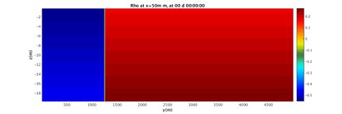
For this tutorial you will be looking at a very simple 2D simulation. A density difference established via a temperature difference begins at a perfect vertical division at t=0s. The division becomes a simple gravity | For this tutorial you will be looking at a very simple 2D simulation. A density difference established via a temperature difference begins at a perfect vertical division at t=0s. The division becomes a simple gravity current as the warmer water floats and the cooler water sinks below. Below is an image of the simulation. You'll note that the boundaries loop around, and that the density differences are driving the gravity current. | ||
[[File:WaveStart.jpg| 500px]] | |||
[[File:WaveCase1.png| 500px]] | [[File:WaveCase1.png| 500px]] | ||
| Line 51: | Line 39: | ||
Go to the ''data_files'' directory and take a look at the contents. One of the most important files there is ''data'' which sets the majority of the important parameters for the MITgcm. The first section of parameters contains a lot of the "fiddly" parameters that you'll want to decide whether or not you need them for your simulation. The MITgcm page "Customizing the Model" will tell you in detail most of the parameters that can be set in ''data''. We will walk through a few of the useful parameters throughout the course of this tutorial. For now, familiarize yourself with the main types according to the PARM section labels. Take special note of the time stepping parameters (&PARM03)-- the ''startTime'' and the ''endTime'' tells you how many iterations the model will run, whereas deltaT is the time in seconds per iteration. | Go to the ''data_files'' directory and take a look at the contents. One of the most important files there is ''data'' which sets the majority of the important parameters for the MITgcm. The first section of parameters contains a lot of the "fiddly" parameters that you'll want to decide whether or not you need them for your simulation. The MITgcm page "Customizing the Model" will tell you in detail most of the parameters that can be set in ''data''. We will walk through a few of the useful parameters throughout the course of this tutorial. For now, familiarize yourself with the main types according to the PARM section labels. Take special note of the time stepping parameters (&PARM03)-- the ''startTime'' and the ''endTime'' tells you how many iterations the model will run, whereas deltaT is the time in seconds per iteration. | ||
''data.pkg'' specifies flags for turning on and off the compiled packages. This should probably match what is | ''data.pkg'' specifies flags for turning on and off the compiled packages. This should probably match what is seen in the ''code/packages.conf'' file if you don't want to be compiling extraneous packages. | ||
All the data files that end with an additional extension are specific to the package in question. For instance ''data.exf'' sets parameters related to the [http://mitgcm.org/public/r2_manual/latest/online_documents/node246.html External Forcing Package]. We will look in detail at ''data.obcs'' in Case 3. | All the data files that end with an additional extension are specific to the package in question. For instance ''data.exf'' sets parameters related to the [http://mitgcm.org/public/r2_manual/latest/online_documents/node246.html External Forcing Package]. We will look in detail at ''data.obcs'' in Case 3. | ||
| Line 73: | Line 61: | ||
% mpirun -np 2 ./mitgcmuv > output < /dev/null & | % mpirun -np 2 ./mitgcmuv > output < /dev/null & | ||
The component ''./mitgcmuv'' runs the executable. The component ''mpirun -np 2'' uses the parallelization MPI on 2 CPU cores. The last segment relays the console output. Note that when you are doing larger-scale, non-tutorial runs (especially when other people are using the machines), you may want to lock on to specific cores. You can look at | The component ''./mitgcmuv'' runs the executable. The component ''mpirun -np 2'' uses the parallelization MPI on 2 CPU cores. The last segment relays the console output. Note that when you are doing larger-scale, non-tutorial runs (especially when other people are using the machines), you may want to lock on to specific cores. You can look at [[Manual_process_placement_on_multi-processor_machines]] to find out how to do that. | ||
For now, run the command: | For now, run the command: | ||
| Line 104: | Line 92: | ||
'''1. Change the grid size from 200x1x40 cells on 2 processors in x to 250x50x40 cells on 4 processors. (must happen at compile-time).''' | '''1. Change the grid size from 200x1x40 cells on 2 processors in x to 250x50x40 cells on 4 processors. (must happen at compile-time).''' | ||
'''2. Change the grid resolution from 25.0m to 20.0 m. Change the time step from 1s/iteration to | '''2. Change the grid resolution from 25.0m to 20.0 m. Change the time step from 1s/iteration to 2s/iteration, and for a length of 12000 seconds. Change the temperature diagnostics to output every 300s.''' | ||
'''3. Place the temperature split at | '''3. Place the temperature split at 2/5 of the domain in x (currently it is at 1/4 of the domain in x)''' | ||
Your simulation will become a 3D simulation! This particular example does not have a lot of three dimensionality, so you will not see significant changes in the experiment behavior. | Your simulation will become a 3D simulation! This particular example does not have a lot of three dimensionality, so you will not see significant changes in the experiment behavior. | ||
| Line 133: | Line 121: | ||
endTime= 6000 => endTime = 12000 | endTime= 6000 => endTime = 12000 | ||
deltaTmom= 1.0 => deltaTmom= | deltaTmom= 1.0 => deltaTmom=2.0 | ||
deltatTtracer=1.0 => deltaTtracer= | deltatTtracer=1.0 => deltaTtracer=2.0 | ||
This edits the time parameters, the end time, and the amount of time per step. Information on the time-stepping in the MITgcm can be found [http://mitgcm.org/public/r2_manual/latest/online_documents/node32.html here]. | This edits the time parameters, the end time, and the amount of time per step. Information on the time-stepping in the MITgcm can be found [http://mitgcm.org/public/r2_manual/latest/online_documents/node32.html here]. | ||
| Line 175: | Line 163: | ||
% Split the domain | % Split the domain | ||
T = ones(nx,ny,nz)*4.0; | T = ones(nx,ny,nz)*4.0; | ||
T2 = ones(nx/ | T2 = ones(nx*2/5,ny,nz)*14; | ||
T(1:nx/ | T(1:nx*2/5, :,:)=T2; | ||
You may want to save this as a new file, however the copy is under source control and this is a pretty minor change. It sometimes is good practice to keep a copy of your generating files in the case folder. As such, copy both the .m and the .bin into the case2 folder. | You may want to save this as a new file, however the copy is under source control and this is a pretty minor change. It sometimes is good practice to keep a copy of your generating files in the case folder. As such, copy both the .m and the .bin into the case2 folder. | ||
| Line 186: | Line 174: | ||
Now that you have 3D data, you can begin looking at slices in different directions. Run the MATLAB script MITgcmGenMovie_Main. This script has a reasonably functional UX and can be used to create basic movies of any 3D MITgcm data (from binary files). Since the script itself should walk you through how to take slices, you are free to play around with different views here. Here are a few examples at certain time slices. | Now that you have 3D data, you can begin looking at slices in different directions. Run the MATLAB script MITgcmGenMovie_Main. This script has a reasonably functional UX and can be used to create basic movies of any 3D MITgcm data (from binary files). Since the script itself should walk you through how to take slices, you are free to play around with different views here. Here are a few examples at certain time slices. | ||
You are encouraged to read the help documentation for the various functions which make up the MITgcmGenMovie_Main script. | You are encouraged to read the help documentation for the various functions which make up the MITgcmGenMovie_Main script. Here are a few example images: | ||
( | Top down view of the simulation at z=0.75m: | ||
[[File:case2_inZ.png| 700px]] | |||
Cutaway in the middle of the simulation (y=25m): | |||
[[File:case2_inY.png|700px]] | |||
It may sometimes come into your interest to place several graphs of different views in the same file. Examine the MATLAB script GenCrossGraphs.m, taking note of how to use the subplot layout. Note that this file manually does the movie stitching, as opposed to using the MITgcmGenGifMovie function. | It may sometimes come into your interest to place several graphs of different views in the same file. Examine the MATLAB script GenCrossGraphs.m, taking note of how to use the subplot layout. Note that this file manually does the movie stitching, as opposed to using the MITgcmGenGifMovie function. | ||
| Line 200: | Line 194: | ||
'''1. Allow open boundary conditions on the east and west.''' | '''1. Allow open boundary conditions on the east and west.''' | ||
'''2. Provide arrays of appropriate length to fit those open boundaries. The eastern open boundary should have a temperature | '''2. Provide arrays of appropriate length to fit those open boundaries. The eastern open boundary should have a temperature of 14C, with a velocity of 1.0m/s. Set the western open boundary with the same values. The western boundary will be the inflow boundary, as the velocity flows from west to east.''' | ||
'''3. Modify the initial temperature array to be a constant 4.0C.''' | '''3. Modify the initial temperature array to be a constant 4.0C.''' | ||
| Line 235: | Line 229: | ||
The first line specifies to create a vector of length 50 (the number of grid cells in y), and place it along the eastern boundary (the -1 wraps around to the last element of the x array). The second specifies a vector of length 50 and places it at the western boundary. | The first line specifies to create a vector of length 50 (the number of grid cells in y), and place it along the eastern boundary (the -1 wraps around to the last element of the x array). The second specifies a vector of length 50 and places it at the western boundary. | ||
Notice how OBSCprescribe is turned on, and different binaries are specified. We'll now need to create those. Save the file and change directories to the input_files directory. If you're familiar with MATLAB or just want to get practice creating binaries using MATLAB, you can try to make your own inflow_outflow.m based on the initial_temperature.m script. It's simply a matter of creating the right arrays | Notice how OBSCprescribe is turned on, and different binaries are specified. We'll now need to create those. Save the file and change directories to the input_files directory. If you're familiar with MATLAB or just want to get practice creating binaries using MATLAB, you can try to make your own inflow_outflow.m based on the initial_temperature.m script. It's simply a matter of creating the right arrays and reading them into files in the same way that the temperature script does. You will note in data.obcs that certain binary file names are specified (you can change these if you like). | ||
If you're in a hurry, simply read through and run the inflow_outflow.m script. Copy the created binaries into your case3 directory. | |||
( | Again, copy the mitgcmuv file you compiled and run the model. You can visualize the data to compare and contrast the differences. | ||
[[File:OpenBCs.png| 700px]] | |||
If you experience model failure, here are a few things you can try: | |||
1. Open up STDERR.* (any of them will do), and read the error messages there. Critical error messages (file not found, mask errors) are printed out in these files. The mask errors are often a result of the outflow and inflow boundary not matching in size. Double check your generating scripts for the binaries if this happens. | |||
2. Open up STDOUT.* and see where the model stopped. (most likely it will be data.obcs) | |||
== Case 4: No Slip BCs and Troubleshooting == | == Case 4: No Slip BCs and Troubleshooting == | ||
The | The overarching purpose of this section is to get familiar with the MIT gcm online code browser, the help documentation, and get into the nitty-gritty of what it means to debug the system. The goal is simple: | ||
'''Activate proper no-slip boundary conditions in the MIT gcm''' | '''Activate proper no-slip boundary conditions in the MIT gcm''' | ||
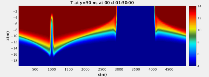
In the following comparison to the IGW, you'll notice that the gravity wave has a more smooth, continuous tail along the bottom boundary as opposed to the non-physical sharp edge of the MIT gcm wave. | |||
[[File:Compare_Example.png]] | [[File:Compare_Example.png]] | ||
When this case is complete, the two cases should match more accurately. The actual process of this case will be very artificial compared to the real procedure of troubleshooting. Nevertheless, hopefully this section may serve as a reference for what to do when unexpected behavior presents itself. | When this case is complete, the two cases should match more accurately. The actual process of this case will be very artificial compared to the real procedure of troubleshooting. Nevertheless, hopefully this section may serve as a reference for what to do when unexpected behavior presents itself. A paper on the mathematics of the implementation of no-slip BCs in the MITgcm can be found [http://wwwf.imperial.ac.uk/~pberloff/OM_deremble_et_al_2011.pdf here] (this is of passing interest but will not necessarily help you to accomplish your goal. | ||
'''A: Initial run and Troubleshooting''' | |||
It is assumed that after getting this far, you know which files are necessary to run the MIT gcm. Copy the data and input files from the case3 folder into the case4 folder (if you have not already) | |||
The first instinct may be to go to the data file and set the following parameters: | |||
no_slip_sides=.FALSE., => no_slip_sides=.TRUE., | |||
no_slip_bottom=.FALSE., => no_slip_bottom=.TRUE., | |||
This would be found after looking at the Customizing the Model page. Give running the model a try after changing these. You may wish to move the endTime back to 6000, as it is clear quite early on whether the boundary conditions are correct. | |||
After running the model, you'll still find the same sharp edge along the boundary conditions. Oh dear! In case you didn't need to troubleshoot at all for case4, now is a good time to look and see if anything is amiss in STDERR or STDOUT. In general STDOUT will not be terribly helpful, as a lot of information is printed to those files. | |||
'''B: Online Help and Digging''' | |||
If you were debugging this as a real issue with your model setup, here are the steps I would recommend (in proper order): | |||
1. Search the MIT gcm website for useful terms. This also searches the MIT gcm Help documentation. | |||
2. Search the MIT gcm code base for the specific parameter no_slip_sides and how it is implemented in the code. Try and track around the code base to see where it comes up. | |||
3. Use Fortran's line-printing to debug which variables are being initialized. If any variables have unexpected initializations, find out why. | |||
Note that 3. is a last resort, however, you would be surprised how much more efficient this may be than 1. in some instances. Below are a few things you may have come across in your travels through each step. If you are pressed for time, you may skip this step or parts of step 3, but know that this section serves as a reference if similar confusing model issues arise in your use of the MITgcm. | |||
'''1. Commentary on available help:''' | |||
[http://mitgcm.org/pipermail/mitgcm-support/2006-November/004477.html Similar issues] appear in this help post. This would give you a clue that the boundary conditions are intimately connected to the vertical viscosity. | |||
'''2. Code Base Navigation:''' | |||
Links from this table would be my starting point for understanding the code. Keep in mind that the online code can sometimes be unreliable as it as not kept as up-to-date as the MITgcm that you may have locally. A good rule of them is to use it as a method of locating the relevant .F files, but checking them on your local copy of the MIT gcm. | |||
Click around in the most relevant areas and search for the variable name you want. Note some weird syntax: Recip generally refers to the reciprocal of an array (division is expensive and often needed, so many of the array reciprocals are stored). The most helpful variables for your issues are usually those which you can eventually link back to INI_PARAMS (otherwise, your issues are with the code itself, and that's a whole other can of worms). | |||
'''3. Printing lines and running the model.''' | |||
The syntax for printing lines in Fortran is: | |||
print *, "My variable: ", my_variable | |||
Keep in mind that Fortran will only work if you have the proper column spacing (6 spaces before any command)! You can find a tutorial on Fortran [http://math.hawaii.edu/wordpress/fortran-1/ here]. With luck you shouldn't have to do much printing lines, though! To investigate what was going wrong I periodically printed sections of arrays in [http://mitgcm.org/public/r2_manual/latest/code_reference/vdb/code/1535.htm#13_L momentum_bottomdrag]. Give this a try, and see if you can figure out how to condition on printing out a specific value based on the Fortran tutorial. | |||
From there I was able to realize that the KappaAR array was all zeroes, which took me to the [http://mitgcm.org/public/r2_manual/latest/code_reference/vdb/code/153.htm#10_L CALC_VISCOSITY] routine. despite being set in the data file. By looking into the code browser again for instances of CALC_VISCOSITY, I was able to find out that this routine is only called if the compile-time parameter [http://mitgcm.org/public/r2_manual/latest/code_reference/vdb/code/183.htm#21_L INCLUDE_CALC_DIFFUSIVITY_CALL] is set! Quite a bit of digging and line-printing. | |||
'''C: Solution''' | |||
In order for the no-slip boundary conditions to work properly, a compile-time flag must be activated. The theme of features needing to be activated ''both'' at compile-time and run-time will no doubt continue to haunt your usage of the MIT gcm. To acquire the proper no-slip boundary conditions, change directories to the ''code'' directory and open CPP_OPTIONS.h. Change the following line: | |||
#undef INCLUDE_CALC_DIFFUSIVITY_CALL => #define INCLUDE_CALC_DIFFUSIVITY_CALL | |||
Recompile, recopy mitgcmuv the executable, run and parse the results! You should now have images that match the IGW boundary conditions in a much more convincing way. | |||
[[File:NoSlip.png|700px]] | |||
For now, that is sufficient for you to start working on your own projects within the MIT gcm. Good luck with your endeavors, and may your model seldom NaN! :) | |||
Latest revision as of 14:57, 28 September 2018
This tutorial is useful if you have never worked with the model before and want to very quickly get a sense of the main parts and offers a "hands on" alternative to sifting through the manual. The tutorial will also attempt to walk you through troubleshooting skills that will be useful as the manual becomes less so. For best results, do attempt the activities before looking at the walkthrough, and take note of references to the MITgcm user manual. Enjoy!
This tutorial assumed you have followed the instructions for setting up the model and for cloning the tutorial code.
Troubleshooting Resources
The MITgcm Online Manual can be found here. A more useful, complete PDF file of the manual can be found here. The MITgcm help support mailing list can be found here, and it is often useful to search the help inquiries (google with the addition site: mitgcm.org) if you are having a specific issue. Finally, the MITgcm is supported by a code browser that allows you to track certain variables within the entire code base. Keep in mind that this search model may contain out-of-date code, but it is a useful resource for sourcing where problems may be found. The best option is always to track it down in your local version of the MITgcm!
Getting Started with the Tutorial
For this tutorial you will need everything in the directory called tutorial wave, and a mpi file for whichever system you are running the MITgcm on. This tutorial does not cover how to write MPI files in order to find your local Fortran compiler, so hopefully you will be provided with one. There are a few mpi-files in the directory mpi_files but they may need revision if the systems have changed since this tutorial was written. The mpi file should be placed in the MITgcm directory tools/build_options
Case 1: Looking at the Example
For this tutorial you will be looking at a very simple 2D simulation. A density difference established via a temperature difference begins at a perfect vertical division at t=0s. The division becomes a simple gravity current as the warmer water floats and the cooler water sinks below. Below is an image of the simulation. You'll note that the boundaries loop around, and that the density differences are driving the gravity current.
A: Compile-Time Procedure
The first course of action is to compile the MITgcm into an executable file. Change directories into the 'build_folder' and run the following command:
% ../../tools/genmake2 -mods=../code -of ../../tools/build_options/my_device_mpi
The first command tells the machine to use genmake2, an MITgcm script for creating all the appropriate make files. The -mods flag tells it where the compile-time options are located. You can cd into ../code if you want to take a look at these. We will address them later. The -of flag locates the mpi file for your particular machine, as mentioned in "getting started". Once genmake2 has concluded use the command:
% make depend
To compile all the Fortran dependencies. The directory should fill up with a large number of .F files. Then use the command:
% make
To complete the creation of the executable. If you have errors they are most likely related to the mpi file at this stage. The error "Clock Skew detected" does not seem to affect the model in any major way. If it completes successfully, you should have an executable called mitgcmuv. Send a copy of this to the directory case_1_density (cp mitgcmuv ../case1_density if you're unfamiliar with Linux). This takes care of all the compile-time information. The main components set at compile time are the grid size (in computational grid cells, not m, see SIZE.h) and which packages are added (see packages.conf). It takes extra time to compile more packages, so don't compile them unless you need them!
B: Run-Time Procedure
Go to the data_files directory and take a look at the contents. One of the most important files there is data which sets the majority of the important parameters for the MITgcm. The first section of parameters contains a lot of the "fiddly" parameters that you'll want to decide whether or not you need them for your simulation. The MITgcm page "Customizing the Model" will tell you in detail most of the parameters that can be set in data. We will walk through a few of the useful parameters throughout the course of this tutorial. For now, familiarize yourself with the main types according to the PARM section labels. Take special note of the time stepping parameters (&PARM03)-- the startTime and the endTime tells you how many iterations the model will run, whereas deltaT is the time in seconds per iteration.
data.pkg specifies flags for turning on and off the compiled packages. This should probably match what is seen in the code/packages.conf file if you don't want to be compiling extraneous packages.
All the data files that end with an additional extension are specific to the package in question. For instance data.exf sets parameters related to the External Forcing Package. We will look in detail at data.obcs in Case 3.
Copy the contents of this directory to case_1_density (cp ./*../case1_density where . means "the directory I am in" and * is a wildcard. You can also use this wildcard to copy and list subsets of other things. For example ls data* should list everything that starts with the string "data". Alright you can get the rest of your regex lesson from the internet...).
Now move yourself to the directory input_files. There should be three MATLAB files inflow_outflow.m, initial_temperature.m, bathymetry.m. You will only need to run initial_temperature.m for now. Open up MATLAB (on hood) using the command matlab
Inside the MATLAB command, open the file using the prompt
>> edit initial_temperature.m
Examine the script and make sure you understand the comments. Then run it in the matlab terminal:
>> initial_temperature
This will create the binary file initial_temp.bin. Copy it and the generating script (all this does is keep a nice record in case you want to look at it again) into the case 1 directory. Change directories to the case 1 directory. You are now ready to run the model!
Once you are in case_1_density run the following command:
% mpirun -np 2 ./mitgcmuv > output < /dev/null &
The component ./mitgcmuv runs the executable. The component mpirun -np 2 uses the parallelization MPI on 2 CPU cores. The last segment relays the console output. Note that when you are doing larger-scale, non-tutorial runs (especially when other people are using the machines), you may want to lock on to specific cores. You can look at Manual_process_placement_on_multi-processor_machines to find out how to do that.
For now, run the command:
% ls T*data
You should start to see one more more files titled T.0000000___.data, each with a number of iterations. These, combined with the .meta files, are the output data of the MITgcm. T is for temperature. Wait until the iterates reach 6000 (this time is set in the data file). Then the model should conclude with the Fortran printout NORMAL END.
C: Data Post-Processing
Using the commands:
 % mv *.data data_processing/
 % mv *.meta data_processing/
Place all the outputted data files in the MATLAB data processing folder. Inside that folder is a number of MATLAB utilities, primarily aimed at creating movies for visualizing the MITgcm data. Open up MATLAB and peruse the file TwoDimensionalRho.m. This takes the density anomaly data from the MITgcm (which is generated by the specified diagnostics file) and plots it as a 2D color plot, from the two times specified in the time manager (it should start from 0 to 6000 in iterates of 100). The code is well commented, so be sure you understand it.
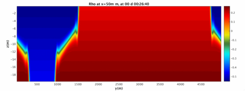
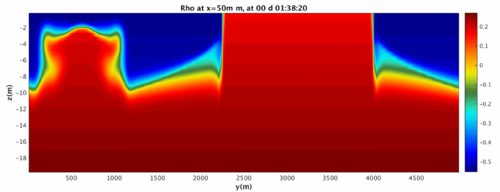
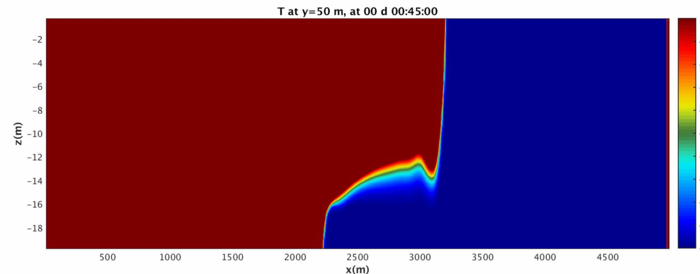
Run the MATLAB script and investigate the folders GIF_IMAGES, GIF_MOVIE, JPG_IMAGES, potentially using xanim to view the movies and display to view the images. The fluid should begin as a split in density on either side that quickly becomes a gravity wave sliding along the bottom surface.
Above is the ending of the gravity wave. Note that because of the wrapping nature of the domain, it changes into a shape not easy to reproduce in a lab! We will address how to turn the domain into a sealed rectangle in case 3.
Congratulations! You've completed your first run of the MIT gcm!
Case 2: Changing the Domain
The goals for this section are as follows. You are encouraged to try to figure them out before looking at the full instructions.
1. Change the grid size from 200x1x40 cells on 2 processors in x to 250x50x40 cells on 4 processors. (must happen at compile-time).
2. Change the grid resolution from 25.0m to 20.0 m. Change the time step from 1s/iteration to 2s/iteration, and for a length of 12000 seconds. Change the temperature diagnostics to output every 300s.
3. Place the temperature split at 2/5 of the domain in x (currently it is at 1/4 of the domain in x)
Your simulation will become a 3D simulation! This particular example does not have a lot of three dimensionality, so you will not see significant changes in the experiment behavior.
A: Compile-Time Procedure
Enter the code directory and open up SIZE.h (you can use vim with the command vi SIZE.h or perhaps gedit with edit SIZE.h. There are parameters for the number of sub-grid points, sub-grids, and processes in X and Y. Notice that the total number of grid points is the product. Make the following changes:
  sNx = 100 => 125
  sNy = 1, => sNy=25,
nPy = 1, => nPy=2,
Keep in mind that the number of processors in x and y is multiplicative as well (nPx=2 , nPy= 2 , total procs=2*2=4). Follow the procedure in the first example to recompile the model. It will overwrite your original mitgcmuv executable, so make sure you've made a copy in the case1 directory. Copy the newly compiled executable into the case2 directory.
Information in the MIT gcm manual on this procedure and the gridding.
B: Run-Time Procedure
Now copy the contents of data_files into case2_domainChange. Change to the case2 directory. Open up the file data and make the following changes:
  delX= 200*25.0 => delX= 250*20.0
  delY= 100.0 => delY= 50*20.0
This changes the grid resolution and accounts for your new grid shape.
  endTime= 6000 => endTime = 12000
  deltaTmom= 1.0 => deltaTmom=2.0
  deltatTtracer=1.0 => deltaTtracer=2.0
This edits the time parameters, the end time, and the amount of time per step. Information on the time-stepping in the MITgcm can be found here.
Save data and open up data.diagnostics. This contains all the information for outputting the binary .data and .meta files. Scroll down and change the line:
#-----------------
 frequency(4) = -100.0,
 timePhase(4) = 0.0,
 fields(1,4)  = 'Theta',
 filename(4)  = 'T',
&
=>
#-----------------
 frequency(4) = -300.0,
 timePhase(4) = 0.0,
 fields(1,4)  = 'Theta',
 filename(4)  = 'T',
&
This changes the output frequency of the temperature data specifically.
Now the input files must be updated to reflect the new domain. Enter the input_files folder and make the following changes to the initial_temperature.m file:
  nx = 200; => nx = 250;
  ny = 1; => ny = 50;
  dx= 25; => dx = 20;
  dy= 100; => dy=20;
This reflects the changes to the resolution and size. Now change the temperature array by switching:
 % Split the domain
 T = ones(nx,ny,nz)*4.0;
 T2 = ones(nx/4,ny,nz)*14;
 T(1:nx/4, :,:)=T2;
=>
 % Split the domain
 T = ones(nx,ny,nz)*4.0;
 T2 = ones(nx*2/5,ny,nz)*14;
 T(1:nx*2/5, :,:)=T2;
You may want to save this as a new file, however the copy is under source control and this is a pretty minor change. It sometimes is good practice to keep a copy of your generating files in the case folder. As such, copy both the .m and the .bin into the case2 folder.
Copy a new version of mitgcmuv from the newly sized build that you compiled in step A. Run the MIT gcm using the same commands as above.
C: Data Post-Processing
Now that you have 3D data, you can begin looking at slices in different directions. Run the MATLAB script MITgcmGenMovie_Main. This script has a reasonably functional UX and can be used to create basic movies of any 3D MITgcm data (from binary files). Since the script itself should walk you through how to take slices, you are free to play around with different views here. Here are a few examples at certain time slices.
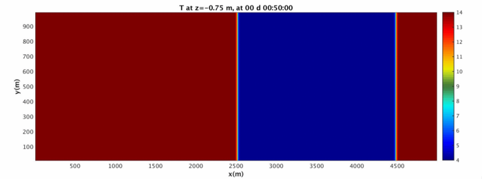
You are encouraged to read the help documentation for the various functions which make up the MITgcmGenMovie_Main script. Here are a few example images:
Top down view of the simulation at z=0.75m:
Cutaway in the middle of the simulation (y=25m):
It may sometimes come into your interest to place several graphs of different views in the same file. Examine the MATLAB script GenCrossGraphs.m, taking note of how to use the subplot layout. Note that this file manually does the movie stitching, as opposed to using the MITgcmGenGifMovie function.
At this point you now should be familiar with how to use MATLAB scripts to interact with the MIT gcm (anything further would fall under the domain of a MATLAB tutorial). The rest of the tutorial will focus on more advanced parameters in the MIT gcm.
Case 3: Using a Package (OBCS)
The goal of this section of the tutorial will be to adjust the simulation from using a pre-set temperature difference to using the Open Boundary Conditions package. You are encouraged to try this out on your own first. Your goals are as follows:
1. Allow open boundary conditions on the east and west.
2. Provide arrays of appropriate length to fit those open boundaries. The eastern open boundary should have a temperature of 14C, with a velocity of 1.0m/s. Set the western open boundary with the same values. The western boundary will be the inflow boundary, as the velocity flows from west to east.
3. Modify the initial temperature array to be a constant 4.0C.
You can read about the package on the MITgcm manual here.
A: Compile-Time Procedure
The first course of action is to add the OBCS package to the list of compiled packages. In the code directory open up packages.conf and add the line obcs (under diagnostics). When adding a new package this will always be necessary. Now open the file OBCS_OPTIONS.h. Make the following changes:
  #undef  ALLOW_OBCS_EAST => #define ALLOW_OBCS_EAST
  #undef ALLOW_OBCS_WEST => #define ALLOW_OBCS_WEST
When you enable a new package, almost all of them will require some form of PKG_OPTIONS.h file for compile-time parameters. The MIT gcm verification directory contains numerous examples which can help you for creating other .h files when compiling other packages.
Compile the code as you would normally.
B: Run-Time Procedure
Copy the data files from Case 2 into the Case 3 directory using the following series of commands (you'll be surprised how often you use these):
  % cp case2_domainChange data* case3_openBC
  % cp case2_domainChange eedata case3_openBC
Enter the case3 directory and first open data.pkg. Add the line:
useOBCS=.TRUE.,
underneath the last package boolean. Like at compile-time, the packages need to be both enabled and specified at run-time. Now open up the file data.obcs, which is analogous to the file OBCS_OPTIONS.h (the same advice applies regarding looking at the verification examples if you need to add on a package that you have no idea how to to specify data files for). Make the following changes to the data.obcs file.
 OB_Ieast= 700*-1, => OB_Ieast=50*-1,
 OB_Iwest= 100*0, => OB_Iwest=50*1,
The first line specifies to create a vector of length 50 (the number of grid cells in y), and place it along the eastern boundary (the -1 wraps around to the last element of the x array). The second specifies a vector of length 50 and places it at the western boundary.
Notice how OBSCprescribe is turned on, and different binaries are specified. We'll now need to create those. Save the file and change directories to the input_files directory. If you're familiar with MATLAB or just want to get practice creating binaries using MATLAB, you can try to make your own inflow_outflow.m based on the initial_temperature.m script. It's simply a matter of creating the right arrays and reading them into files in the same way that the temperature script does. You will note in data.obcs that certain binary file names are specified (you can change these if you like).
If you're in a hurry, simply read through and run the inflow_outflow.m script. Copy the created binaries into your case3 directory.
Again, copy the mitgcmuv file you compiled and run the model. You can visualize the data to compare and contrast the differences.
If you experience model failure, here are a few things you can try:
1. Open up STDERR.* (any of them will do), and read the error messages there. Critical error messages (file not found, mask errors) are printed out in these files. The mask errors are often a result of the outflow and inflow boundary not matching in size. Double check your generating scripts for the binaries if this happens. 2. Open up STDOUT.* and see where the model stopped. (most likely it will be data.obcs)
Case 4: No Slip BCs and Troubleshooting
The overarching purpose of this section is to get familiar with the MIT gcm online code browser, the help documentation, and get into the nitty-gritty of what it means to debug the system. The goal is simple:
Activate proper no-slip boundary conditions in the MIT gcm
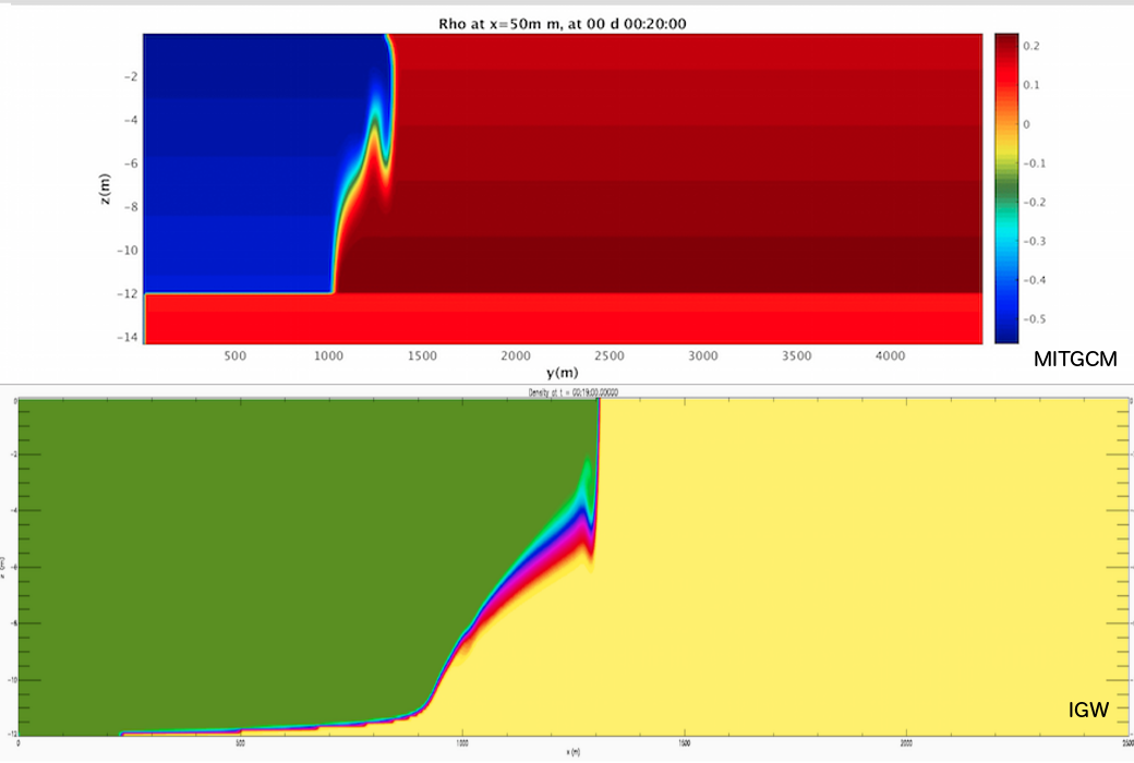
In the following comparison to the IGW, you'll notice that the gravity wave has a more smooth, continuous tail along the bottom boundary as opposed to the non-physical sharp edge of the MIT gcm wave.
When this case is complete, the two cases should match more accurately. The actual process of this case will be very artificial compared to the real procedure of troubleshooting. Nevertheless, hopefully this section may serve as a reference for what to do when unexpected behavior presents itself. A paper on the mathematics of the implementation of no-slip BCs in the MITgcm can be found here (this is of passing interest but will not necessarily help you to accomplish your goal.
A: Initial run and Troubleshooting
It is assumed that after getting this far, you know which files are necessary to run the MIT gcm. Copy the data and input files from the case3 folder into the case4 folder (if you have not already)
The first instinct may be to go to the data file and set the following parameters:
  no_slip_sides=.FALSE., => no_slip_sides=.TRUE.,
  no_slip_bottom=.FALSE., => no_slip_bottom=.TRUE.,
This would be found after looking at the Customizing the Model page. Give running the model a try after changing these. You may wish to move the endTime back to 6000, as it is clear quite early on whether the boundary conditions are correct.
After running the model, you'll still find the same sharp edge along the boundary conditions. Oh dear! In case you didn't need to troubleshoot at all for case4, now is a good time to look and see if anything is amiss in STDERR or STDOUT. In general STDOUT will not be terribly helpful, as a lot of information is printed to those files.
B: Online Help and Digging
If you were debugging this as a real issue with your model setup, here are the steps I would recommend (in proper order):
1. Search the MIT gcm website for useful terms. This also searches the MIT gcm Help documentation.
2. Search the MIT gcm code base for the specific parameter no_slip_sides and how it is implemented in the code. Try and track around the code base to see where it comes up.
3. Use Fortran's line-printing to debug which variables are being initialized. If any variables have unexpected initializations, find out why.
Note that 3. is a last resort, however, you would be surprised how much more efficient this may be than 1. in some instances. Below are a few things you may have come across in your travels through each step. If you are pressed for time, you may skip this step or parts of step 3, but know that this section serves as a reference if similar confusing model issues arise in your use of the MITgcm.
1. Commentary on available help:
Similar issues appear in this help post. This would give you a clue that the boundary conditions are intimately connected to the vertical viscosity.
2. Code Base Navigation:
Links from this table would be my starting point for understanding the code. Keep in mind that the online code can sometimes be unreliable as it as not kept as up-to-date as the MITgcm that you may have locally. A good rule of them is to use it as a method of locating the relevant .F files, but checking them on your local copy of the MIT gcm.
Click around in the most relevant areas and search for the variable name you want. Note some weird syntax: Recip generally refers to the reciprocal of an array (division is expensive and often needed, so many of the array reciprocals are stored). The most helpful variables for your issues are usually those which you can eventually link back to INI_PARAMS (otherwise, your issues are with the code itself, and that's a whole other can of worms).
3. Printing lines and running the model.
The syntax for printing lines in Fortran is:
print *, "My variable: ", my_variable
Keep in mind that Fortran will only work if you have the proper column spacing (6 spaces before any command)! You can find a tutorial on Fortran here. With luck you shouldn't have to do much printing lines, though! To investigate what was going wrong I periodically printed sections of arrays in momentum_bottomdrag. Give this a try, and see if you can figure out how to condition on printing out a specific value based on the Fortran tutorial.
From there I was able to realize that the KappaAR array was all zeroes, which took me to the CALC_VISCOSITY routine. despite being set in the data file. By looking into the code browser again for instances of CALC_VISCOSITY, I was able to find out that this routine is only called if the compile-time parameter INCLUDE_CALC_DIFFUSIVITY_CALL is set! Quite a bit of digging and line-printing.
C: Solution
In order for the no-slip boundary conditions to work properly, a compile-time flag must be activated. The theme of features needing to be activated both at compile-time and run-time will no doubt continue to haunt your usage of the MIT gcm. To acquire the proper no-slip boundary conditions, change directories to the code directory and open CPP_OPTIONS.h. Change the following line:
#undef INCLUDE_CALC_DIFFUSIVITY_CALL => #define INCLUDE_CALC_DIFFUSIVITY_CALL
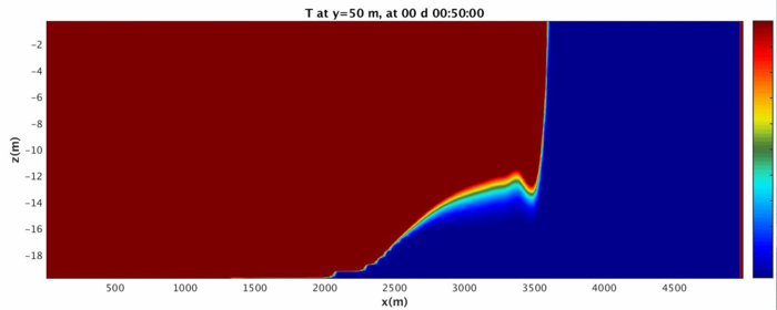
Recompile, recopy mitgcmuv the executable, run and parse the results! You should now have images that match the IGW boundary conditions in a much more convincing way.
For now, that is sufficient for you to start working on your own projects within the MIT gcm. Good luck with your endeavors, and may your model seldom NaN! :)
