Energy Budget: Difference between revisions
(Created page with "The energy budget for a density-stratified Boussinesq fluid was first discussed by Winters et al. in 1995. We will largely follow their notation and conceptual framework. In...") |
mNo edit summary |
||
| (One intermediate revision by the same user not shown) | |||
| Line 1: | Line 1: | ||
The energy budget for a density-stratified Boussinesq fluid was first discussed by Winters et al. | The energy budget for a density-stratified Boussinesq fluid was first discussed by Winters et al. (1995). We will largely follow their notation and conceptual framework. | ||
The following will ignore surface fluxes or additional body forces (like tides or rotation). Addition of these terms is not difficult, but since these situations do not arise much (as yet) in the research projects at UW, we will not include them here. | |||
| Line 20: | Line 20: | ||
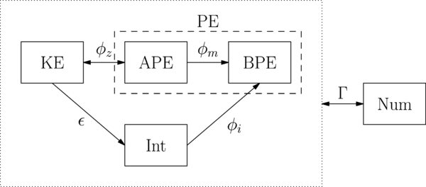
Graphically, this looks like: | Graphically, this looks like: | ||
[[File:energy_budget.png|600px|]] | |||
where Num is the energy lost/gained due to the numerical model/scheme/filter. | |||
All the energy components are: | All the energy components are: | ||
| Line 43: | Line 44: | ||
|APE | |APE | ||
|<math> \text{PE} - \text{BPE} </math> | |<math> \text{PE} - \text{BPE} </math> | ||
|No | |||
|- | |||
|ME | |||
|<math> \text{KE} + \text{PE} </math> | |||
|No | |No | ||
|} | |} | ||
| Line 74: | Line 79: | ||
|} | |} | ||
The energy components and conversion rates | The rates of change of each component are | ||
<math> \begin{align} | |||
\frac{d\text{KE}}{dt} &= -\phi_z - \epsilon\\ | |||
\frac{d\text{APE}}{dt} &= \phi_z - \phi_m\\ | |||
\frac{d\text{BPE}}{dt} &= \phi_m + \phi_i\\ | |||
\frac{d\text{Int}}{dt} &= \epsilon - \phi_i | |||
\end{align} | |||
</math> | |||
Including the rate of energy added/subtracted due to the numerical model or the filter, <math>\Gamma</math>, the evolution equation of the total mechanical energy is | |||
<math> \frac{d ME}{dt} = \phi_i - \epsilon - \Gamma </math> | |||
The energy components and conversion rates that are not computed live in spins (as well as the energy lost to numerics) are computed in post using Matlab in the plot_diagnos.m function in [[SPINS MATLAB tools]]. SPINS returns enough budget information for the uncomputed variables to be evaluated from the above definitions. | |||
Latest revision as of 16:03, 8 October 2020
The energy budget for a density-stratified Boussinesq fluid was first discussed by Winters et al. (1995). We will largely follow their notation and conceptual framework.
The following will ignore surface fluxes or additional body forces (like tides or rotation). Addition of these terms is not difficult, but since these situations do not arise much (as yet) in the research projects at UW, we will not include them here.
The energy within the system can be broken down into the follow categories
| Mechanical Energy (ME) | Internal Energy (Int) | ||
|---|---|---|---|
| Kinetic (KE) | Potential (PE) | ||
| APE | BPE | ||
Graphically, this looks like:
where Num is the energy lost/gained due to the numerical model/scheme/filter.
All the energy components are:
| Component | Definition | computed live in SPINS? |
|---|---|---|
| KE | Yes | |
| PE | Yes | |
| BPE | Yes | |
| APE | No | |
| ME | No |
where is the depth of an element of the sorted density field which minimized the potential energy.
The definitions for the energy conversion rates are:
| Rate | Definition | computed live in SPINS? |
|---|---|---|
| Yes | ||
| No | ||
| No | ||
| Yes | ||
| No |
The rates of change of each component are
Including the rate of energy added/subtracted due to the numerical model or the filter, , the evolution equation of the total mechanical energy is
The energy components and conversion rates that are not computed live in spins (as well as the energy lost to numerics) are computed in post using Matlab in the plot_diagnos.m function in SPINS MATLAB tools. SPINS returns enough budget information for the uncomputed variables to be evaluated from the above definitions.


