stat946w18/Self Normalizing Neural Networks
Introduction and Motivation
While neural networks have been making a lot of headway in improving benchmark results and narrowing the gap with human-level performance, success has been fairly limited to visual and sequential processing tasks through advancements in convolutional network and recurrent network structures. Most data science competitions outside of these domains are still outperformed by algorithms such as gradient boosting and random forests. The traditional (densely connected) feed-forward neural networks (FNNs) are rarely used competitively, and when they do win on rare occasions, they have very shallow network architectures with just up to four layers [10].
The authors, Klambauer et al., believe that what prevents FNNs from becoming more competitively useful is the inability to train a deeper FNN structure, which would allow the network to learn more levels of abstract representations. Primarily, the difficulty arises due to the instability of gradients in very deep FNNs leading to problems like gradient vanishing/explosion. To have a deeper network, oscillations in the distribution of activations need to be kept under control so that stable gradients can be obtained during training. Several techniques are available to normalize activations, including batch normalization [6], layer normalization [1] and weight normalization [8]. These methods work well with CNNs and RNNs, but not so much with FNNs because backpropagating through normalization parameters introduces additional variance to the gradients, and regularization techniques like dropout further perturb the normalization effect. CNNs and RNNs are less sensitive to such perturbations, presumably due to their weight sharing architecture, but FNNs do not have such a property and thus suffer from high variance in training errors, which hinders learning. Furthermore, the aforementioned normalization techniques involve adding external layers to the model and can slow down computation, which may already be slow when working with very deep FNNs.
Therefore, the authors were motivated to develop a new FNN implementation that can achieve the intended effect of normalization techniques that works well with stochastic gradient descent and dropout. Self-normalizing neural networks (SNNs) are based on the idea of scaled exponential linear units (SELU), a new activation function introduced in this paper, whose output distribution is proved to converge to a fixed point, thus making it possible to train deeper networks.
Notations
As the paper (primarily in the supplementary materials) comes with lengthy proofs, important notations are listed first.
Consider two fully-connected layers, let [math]\displaystyle{ x }[/math] denote the inputs to the second layer, then [math]\displaystyle{ z = Wx }[/math] represents the network inputs of the second layer, and [math]\displaystyle{ y = f(z) }[/math] represents the activations in the second layer.
Assume that all activations from a lower layer [math]\displaystyle{ x_i }[/math]'s, [math]\displaystyle{ 1 \leqslant i \leqslant n }[/math], have the same mean [math]\displaystyle{ \mu := \mathrm{E}(x_i) }[/math] and the same variance [math]\displaystyle{ \nu := \mathrm{Var}(x_i) }[/math] and that each [math]\displaystyle{ y }[/math] has mean [math]\displaystyle{ \widetilde{\mu} := \mathrm{E}(y) }[/math] and variance [math]\displaystyle{ \widetilde{\nu} := \mathrm{Var}(y) }[/math], then let [math]\displaystyle{ g }[/math] be the set of functions that maps [math]\displaystyle{ (\mu, \nu) }[/math] to [math]\displaystyle{ (\widetilde{\mu}, \widetilde{\nu}) }[/math].
For the weight vector [math]\displaystyle{ w }[/math], [math]\displaystyle{ n }[/math] times the mean of the weight vector is [math]\displaystyle{ \omega := \sum_{i = 1}^n \omega_i }[/math] and [math]\displaystyle{ n }[/math] times the second moment is [math]\displaystyle{ \tau := \sum_{i = 1}^{n} w_i^2 }[/math].
Key Concepts
Self-Normalizing Neural-Net (SNN)
A neural network is self-normalizing if it possesses a mapping [math]\displaystyle{ g: \Omega \rightarrow \Omega }[/math] for each activation [math]\displaystyle{ y }[/math] that maps mean and variance from one layer to the next and has a stable and attracting fixed point depending on [math]\displaystyle{ (\omega, \tau) }[/math] in [math]\displaystyle{ \Omega }[/math]. Furthermore, the mean and variance remain in the domain [math]\displaystyle{ \Omega }[/math], that is [math]\displaystyle{ g(\Omega) \subseteq \Omega }[/math], where [math]\displaystyle{ \Omega = \{ (\mu, \nu) | \mu \in [\mu_{min}, \mu_{max}], \nu \in [\nu_{min}, \nu_{max}] \} }[/math]. When iteratively applying the mapping [math]\displaystyle{ g }[/math], each point within [math]\displaystyle{ \Omega }[/math] converges to this fixed point.
In other words, in SNNs, if the inputs from an earlier layer ([math]\displaystyle{ x }[/math]) already have their mean and variance within a predefined interval [math]\displaystyle{ \Omega }[/math], then the activations to the next layer ([math]\displaystyle{ y = f(z = Wx) }[/math]) should remain within those intervals. This is true across all pairs of connecting layers as the normalizing effect gets propagated through the network, hence why the term self-normalizing. When the mapping is applied iteratively, it should draw the mean and variance values closer to a fixed point within [math]\displaystyle{ \Omega }[/math], the value of which depends on [math]\displaystyle{ \omega }[/math] and [math]\displaystyle{ \tau }[/math] (recall that they are from the weight vector).
We will design a FNN then construct a g that takes the mean and variance of each layer to those of the next and is a contraction mapping i.e. [math]\displaystyle{ g(\mu_i, \nu_i) = (\mu_{i+1}, \nu_{i+1}) \forall i }[/math]. It should be noted that although the g required in the SNN definition depends on [math]\displaystyle{ (\omega, \tau) }[/math] of an individual layer, the FNN that we construct will have the same values of [math]\displaystyle{ (\omega, \tau) }[/math] for each layer. Intuitively this definition can be interpreted as saying that the mean and variance of the final layer of a sufficiently deep SNN will not change when the mean and variance of the input data change. This is because the mean and variance are passing through a contraction mapping at each layer, converging to the mapping's fixed point.
The activation function that makes an SNN possible should meet the following four conditions:
- It can take on both negative and positive values, so it can normalize the mean;
- It has a saturation region, so it can dampen variances that are too large;
- It has a slope larger than one, so it can increase variances that are too small; and
- It is a continuous curve, which is necessary for the fixed point to exist (see the definition of Banach fixed point theorem to follow).
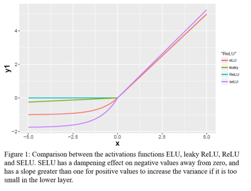
Commonly used activation functions such as rectified linear units (ReLU), sigmoid, tanh, leaky ReLUs and exponential linear units (ELUs) do not meet all four criteria, therefore, a new activation function is needed.
Scaled Exponential Linear Units (SELUs)
One of the main ideas introduced in this paper is the SELU function. As the name suggests, it is closely related to ELU [3],
\[ \mathrm{elu}(x) = \begin{cases} x & x > 0 \\ \alpha e^x - \alpha & x \leqslant 0 \end{cases} \]
but further builds upon it by introducing a new scale parameter $\lambda$ and proving the exact values that $\alpha$ and $\lambda$ should take on to achieve self-normalization. SELU is defined as:
\[ \mathrm{selu}(x) = \lambda \begin{cases} x & x > 0 \\ \alpha e^x - \alpha & x \leqslant 0 \end{cases} \]
SELUs meet all four criteria listed above - it takes on positive values when [math]\displaystyle{ x \gt 0 }[/math] and negative values when [math]\displaystyle{ x \lt 0 }[/math], it has a saturation region when [math]\displaystyle{ x }[/math] is a larger negative value, the value of [math]\displaystyle{ \lambda }[/math] can be set to greater than one to ensure a slope greater than one, and it is continuous at [math]\displaystyle{ x = 0 }[/math].
Figure 1 below gives an intuition for how SELUs normalize activations across layers. As shown, a variance dampening effect occurs when inputs are negative and far away from zero, and a variance increasing effect occurs when inputs are close to zero.
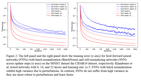
Figure 2 below plots the progression of training error on the MNIST and CIFAR10 datasets when training with SNNs versus FNNs with batch normalization at varying model depths. As shown, FNNs that adopted the SELU activation function exhibited lower and less variable training loss compared to using batch normalization, even as the depth increased to 16 and 32 layers.
Banach Fixed Point Theorem and Contraction Mappings
The underlying theory behind SNNs is the Banach fixed point theorem, which states the following: Let [math]\displaystyle{ (X, d) }[/math] be a non-empty complete metric space with a contraction mapping [math]\displaystyle{ f: X \rightarrow X }[/math]. Then [math]\displaystyle{ f }[/math] has a unique fixed point [math]\displaystyle{ x_f \subseteq X }[/math] with [math]\displaystyle{ f(x_f) = x_f }[/math]. Every sequence [math]\displaystyle{ x_n = f(x_{n-1}) }[/math] with starting element [math]\displaystyle{ x_0 \subseteq X }[/math] converges to the fixed point: [math]\displaystyle{ x_n \underset{n \rightarrow \infty}\rightarrow x_f }[/math].
A contraction mapping is a function [math]\displaystyle{ f: X \rightarrow X }[/math] on a metric space [math]\displaystyle{ X }[/math] with distance [math]\displaystyle{ d }[/math], such that for all points [math]\displaystyle{ \mathbf{u} }[/math] and [math]\displaystyle{ \mathbf{v} }[/math] in [math]\displaystyle{ X }[/math]: [math]\displaystyle{ d(f(\mathbf{u}), f(\mathbf{v})) \leqslant \delta d(\mathbf{u}, \mathbf{v}) }[/math], for a [math]\displaystyle{ 0 \leqslant \delta \leqslant 1 }[/math].
The easiest way to prove a contraction mapping is usually to show that the spectral norm [12] of its Jacobian is less than 1 [13], as was done for this paper.
Proving the Self-Normalizing Property
Mean and Variance Mapping Function
[math]\displaystyle{ g }[/math] is derived under the assumption that [math]\displaystyle{ x_i }[/math]'s are independent but not necessarily having the same mean and variance (2). Under this assumption (and recalling earlier notation of [math]\displaystyle{ \omega }[/math] and [math]\displaystyle{ \tau }[/math]),
\begin{align} \mathrm{E}(z = \mathbf{w}^T \mathbf{x}) = \sum_{i = 1}^n w_i \mathrm{E}(x_i) = \mu \omega \end{align}
\begin{align} \mathrm{Var}(z) = \mathrm{Var}(\sum_{i = 1}^n w_i x_i) = \sum_{i = 1}^n w_i^2 \mathrm{Var}(x_i) = \nu \sum_{i = 1}^n w_i^2 = \nu\tau \textrm{ .} \end{align}
When the weight terms are normalized, [math]\displaystyle{ z }[/math] can be viewed as a weighted sum of [math]\displaystyle{ x_i }[/math]'s. Wide neural net layers with a large number of nodes is common, so [math]\displaystyle{ n }[/math] is usually large, and by the Central Limit Theorem, [math]\displaystyle{ z }[/math] approaches a normal distribution [math]\displaystyle{ \mathcal{N}(\mu\omega, \sqrt{\nu\tau}) }[/math].
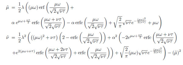
Using the above property, the exact form for [math]\displaystyle{ g }[/math] can be obtained using the definitions for mean and variance of continuous random variables:

Analytical solutions for the integrals can be obtained as follows:
The authors are interested in the fixed point [math]\displaystyle{ (\mu, \nu) = (0, 1) }[/math] as these are the parameters associated with the common standard normal distribution. The authors also proposed using normalized weights such that [math]\displaystyle{ \omega = \sum_{i = 1}^n = 0 }[/math] and [math]\displaystyle{ \tau = \sum_{i = 1}^n w_i^2= 1 }[/math] as it gives a simpler, cleaner expression for [math]\displaystyle{ \widetilde{\mu} }[/math] and [math]\displaystyle{ \widetilde{\nu} }[/math] in the calculations in the next steps. This weight scheme can be achieved in several ways, for example, by drawing from a normal distribution [math]\displaystyle{ \mathcal{N}(0, \frac{1}{n}) }[/math] or from a uniform distribution [math]\displaystyle{ U(-\sqrt{3}, \sqrt{3}) }[/math].
At [math]\displaystyle{ \widetilde{\mu} = \mu = 0 }[/math], [math]\displaystyle{ \widetilde{\nu} = \nu = 1 }[/math], [math]\displaystyle{ \omega = 0 }[/math] and [math]\displaystyle{ \tau = 1 }[/math], the constants [math]\displaystyle{ \lambda }[/math] and [math]\displaystyle{ \alpha }[/math] from the SELU function can be solved for - [math]\displaystyle{ \lambda_{01} \approx 1.0507 }[/math] and [math]\displaystyle{ \alpha_{01} \approx 1.6733 }[/math]. These values are used throughout the rest of the paper whenever an expression calls for [math]\displaystyle{ \lambda }[/math] and [math]\displaystyle{ \alpha }[/math].
Details of Moment-Mapping Integrals
Consider the moment-mapping integrals: \begin{align} \widetilde{\mu} & = \int_{-\infty}^\infty \mathrm{selu} (z) p_N(z; \mu \omega, \sqrt{\nu \tau})dz\\ \widetilde{\nu} & = \int_{-\infty}^\infty \mathrm{selu} (z)^2 p_N(z; \mu \omega, \sqrt{\nu \tau}) dz-\widetilde{\mu}^2. \end{align}
The equation for [math]\displaystyle{ \widetilde{\mu} }[/math] can be expanded as \begin{align} \widetilde{\mu} & = \frac{\lambda}{2}\left( 2\alpha\int_{-\infty}^0 (\exp(z)-1) p_N(z; \mu \omega, \sqrt{\nu \tau})dz +2\int_{0}^\infty z p_N(z; \mu \omega, \sqrt{\nu \tau})dz \right)\\ &= \frac{\lambda}{2}\left( 2 \alpha \frac{1}{\sqrt{2\pi\tau\nu}} \int_{-\infty}^0 (\exp(z)-1) \exp(\frac{-1}{2\tau \nu} (z-\mu \omega)^2 ) dz +2\frac{1}{\sqrt{2\pi\tau\nu}}\int_{0}^\infty z \exp(\frac{-1}{2\tau \nu} (z-\mu \omega)^2 dz \right)\\ &= \frac{\lambda}{2}\left( 2 \alpha\frac{1}{\sqrt{2\pi\tau\nu}}\int_{-\infty}^0 \exp(z) \exp(\frac{-1}{2\tau \nu} (z-\mu \omega)^2 ) dz - 2 \alpha\frac{1}{\sqrt{2\pi\tau\nu}}\int_{-\infty}^0 \exp(\frac{-1}{2\tau \nu} (z-\mu \omega)^2 ) dz +2\frac{1}{\sqrt{2\pi\tau\nu}}\int_{0}^\infty z \exp(\frac{-1}{2\tau \nu} (z-\mu \omega)^2 dz \right)\\ \end{align}
The first integral can be simplified via the substituiton \begin{align} q:= \frac{1}{\sqrt{2\tau \nu}}(z-\mu \omega -\tau \nu). \end{align} While the second and third can be simplified via the substitution \begin{align} q:= \frac{1}{\sqrt{2\tau \nu}}(z-\mu \omega ). \end{align} Using the definitions of [math]\displaystyle{ \mathrm{erf} }[/math] and [math]\displaystyle{ \mathrm{erfc} }[/math] then yields the result of the previous section.
Self-Normalizing Property Under Normalized Weights
Assuming the the weights normalized with [math]\displaystyle{ \omega=0 }[/math] and [math]\displaystyle{ \tau=1 }[/math], it is possible to calculate the exact value for the spectral norm [12] of [math]\displaystyle{ g }[/math]'s Jacobian around the fixed point [math]\displaystyle{ (\mu, \nu) = (0, 1) }[/math], which turns out to be [math]\displaystyle{ 0.7877 }[/math]. Thus, at initialization, SNNs have a stable and attracting fixed point at [math]\displaystyle{ (0, 1) }[/math], which means that when [math]\displaystyle{ g }[/math] is applied iteratively to a pair [math]\displaystyle{ (\mu_{new}, \nu_{new}) }[/math], it should draw the points closer to [math]\displaystyle{ (0, 1) }[/math]. The rate of convergence is determined by the spectral norm [12], whose value depends on [math]\displaystyle{ \mu }[/math], [math]\displaystyle{ \nu }[/math], [math]\displaystyle{ \omega }[/math] and [math]\displaystyle{ \tau }[/math].

Self-Normalizing Property Under Unnormalized Weights
As weights are updated during training, there is no guarantee that they would remain normalized. The authors addressed this issue through the first key theorem presented in the paper, which states that a fixed point close to (0, 1) can still be obtained if [math]\displaystyle{ \mu }[/math], [math]\displaystyle{ \nu }[/math], [math]\displaystyle{ \omega }[/math] and [math]\displaystyle{ \tau }[/math] are restricted to a specified range.
Additionally, there is no guarantee that the mean and variance of the inputs would stay within the range given by the first theorem, which led to the development of theorems #2 and #3. These two theorems established an upper and lower bound on the variance of inputs if the variance of activations from the previous layer are above or below the range specified, respectively. This ensures that the variance would not explode or vanish after being propagated through the network.
The theorems come with lengthy proofs in the supplementary materials for the paper. High-level proof sketches are presented here.
Theorem 1: Stable and Attracting Fixed Points Close to (0, 1)
Definition: We assume [math]\displaystyle{ \alpha = \alpha_{01} }[/math] and [math]\displaystyle{ \lambda = \lambda_{01} }[/math]. We restrict the range of the variables to the domain [math]\displaystyle{ \mu \in [-0.1, 0.1] }[/math], [math]\displaystyle{ \omega \in [-0.1, 0.1] }[/math], [math]\displaystyle{ \nu \in [0.8, 1.5] }[/math], and [math]\displaystyle{ \tau \in [0.9, 1.1] }[/math]. For [math]\displaystyle{ \omega = 0 }[/math] and [math]\displaystyle{ \tau = 1 }[/math], the mapping has the stable fixed point [math]\displaystyle{ (\mu, \nu) = (0, 1 }[/math]. For other [math]\displaystyle{ \omega }[/math] and [math]\displaystyle{ \tau }[/math], g has a stable and attracting fixed point depending on [math]\displaystyle{ (\omega, \tau) }[/math] in the [math]\displaystyle{ (\mu, \nu) }[/math]-domain: [math]\displaystyle{ \mu \in [-0.03106, 0.06773] }[/math] and [math]\displaystyle{ \nu \in [0.80009, 1.48617] }[/math]. All points within the [math]\displaystyle{ (\mu, \nu) }[/math]-domain converge when iteratively applying the mapping to this fixed point.
Proof: In order to show the the mapping [math]\displaystyle{ g }[/math] has a stable and attracting fixed point close to [math]\displaystyle{ (0, 1) }[/math], the authors again applied Banach's fixed point theorem, which states that a contraction mapping on a nonempty complete metric space that does not map outside its domain has a unique fixed point, and that all points in the [math]\displaystyle{ (\mu, \nu) }[/math]-domain converge to the fixed point when [math]\displaystyle{ g }[/math] is iteratively applied.
The two requirements are proven as follows:
1. g is a contraction mapping.
For [math]\displaystyle{ g }[/math] to be a contraction mapping in [math]\displaystyle{ \Omega }[/math] with distance [math]\displaystyle{ ||\cdot||_2 }[/math], there must exist a Lipschitz constant [math]\displaystyle{ M \lt 1 }[/math] such that:
\begin{align} \forall \mu, \nu \in \Omega: ||g(\mu) - g(\nu)||_2 \leqslant M||\mu - \nu||_2 \end{align}
As stated earlier, [math]\displaystyle{ g }[/math] is a contraction mapping if the spectral norm [12] of the Jacobian [math]\displaystyle{ \mathcal{H} }[/math] (3) is below one, or equivalently, if the the largest singular value of [math]\displaystyle{ \mathcal{H} }[/math] is less than 1.
To find the singular values of [math]\displaystyle{ \mathcal{H} }[/math], the authors used an explicit formula derived by Blinn [2] for [math]\displaystyle{ 2\times2 }[/math] matrices, which states that the largest singular value of the matrix is [math]\displaystyle{ \frac{1}{2}(\sqrt{(a_{11} + a_{22}) ^ 2 + (a_{21} - a{12})^2} + \sqrt{(a_{11} - a_{22}) ^ 2 + (a_{21} + a{12})^2}) }[/math].
For [math]\displaystyle{ \mathcal{H} }[/math], an expression for the largest singular value of [math]\displaystyle{ \mathcal{H} }[/math], made up of the first-order partial derivatives of the mapping [math]\displaystyle{ g }[/math] with respect to [math]\displaystyle{ \mu }[/math] and [math]\displaystyle{ \nu }[/math], can be derived given the analytical solutions for [math]\displaystyle{ \widetilde{\mu} }[/math] and [math]\displaystyle{ \widetilde{\nu} }[/math] (and denoted [math]\displaystyle{ S(\mu, \omega, \nu, \tau, \lambda, \alpha) }[/math]).
From the mean value theorem, we know that for a [math]\displaystyle{ t \in [0, 1] }[/math],
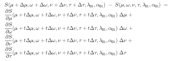
Therefore, the distance of the singular value at [math]\displaystyle{ S(\mu, \omega, \nu, \tau, \lambda_{\mathrm{01}}, \alpha_{\mathrm{01}}) }[/math] and at [math]\displaystyle{ S(\mu + \Delta\mu, \omega + \Delta\omega, \nu + \Delta\nu, \tau \Delta\tau, \lambda_{\mathrm{01}}, \alpha_{\mathrm{01}}) }[/math] can be bounded above by
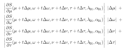
An upper bound was obtained for each partial derivative term above, mainly through algebraic reformulations and by making use of the fact that many of the functions are monotonically increasing or decreasing on the variables they depend on in [math]\displaystyle{ \Omega }[/math] (see pages 17 - 25 in the supplementary materials).
The [math]\displaystyle{ \Delta }[/math] terms were then set (rather arbitrarily) to be: [math]\displaystyle{ \Delta \mu=0.0068097371 }[/math], [math]\displaystyle{ \Delta \omega=0.0008292885 }[/math], [math]\displaystyle{ \Delta \nu=0.0009580840 }[/math], and [math]\displaystyle{ \Delta \tau=0.0007323095 }[/math]. Plugging in the upper bounds on the absolute values of the derivative terms for [math]\displaystyle{ S }[/math] and the [math]\displaystyle{ \Delta }[/math] terms yields
\[ S(\mu + \Delta \mu,\omega + \Delta \omega,\nu + \Delta \nu,\tau + \Delta \tau,\lambda_{\rm 01},\alpha_{\rm 01}) - S(\mu,\omega,\nu,\tau,\lambda_{\rm 01},\alpha_{\rm 01}) < 0.008747 \]
Next, the largest singular value is found from a computer-assisted fine grid-search (1) over the domain [math]\displaystyle{ \Omega }[/math], with grid lengths [math]\displaystyle{ \Delta \mu=0.0068097371 }[/math], [math]\displaystyle{ \Delta \omega=0.0008292885 }[/math], [math]\displaystyle{ \Delta \nu=0.0009580840 }[/math], and [math]\displaystyle{ \Delta \tau=0.0007323095 }[/math], which turned out to be [math]\displaystyle{ 0.9912524171058772 }[/math]. Therefore,
\[ S(\mu + \Delta \mu,\omega + \Delta \omega,\nu + \Delta \nu,\tau + \Delta \tau,\lambda_{\rm 01},\alpha_{\rm 01}) \leq 0.9912524171058772 + 0.008747 < 1 \]
Since the largest singular value is smaller than 1, [math]\displaystyle{ g }[/math] is a contraction mapping.
2. g does not map outside its domain.
To prove that [math]\displaystyle{ g }[/math] does not map outside of the domain [math]\displaystyle{ \mu \in [-0.1, 0.1] }[/math] and [math]\displaystyle{ \nu \in [0.8, 1.5] }[/math], lower and upper bounds on [math]\displaystyle{ \widetilde{\mu} }[/math] and [math]\displaystyle{ \widetilde{\nu} }[/math] were obtained to show that they stay within [math]\displaystyle{ \Omega }[/math].
First, it was shown that the derivatives of [math]\displaystyle{ \widetilde{\mu} }[/math] and [math]\displaystyle{ \widetilde{\xi} }[/math] with respect to [math]\displaystyle{ \mu }[/math] and [math]\displaystyle{ \nu }[/math] are either positive or have the sign of [math]\displaystyle{ \omega }[/math] in [math]\displaystyle{ \Omega }[/math], so the minimum and maximum points are found at the borders. In [math]\displaystyle{ \Omega }[/math], it then follows that
\begin{align} -0.03106 <\widetilde{\mu}(-0.1,0.1, 0.8, 0.95, \lambda_{\rm 01}, \alpha_{\rm 01}) \leq & \widetilde{\mu} \leq \widetilde{\mu}(0.1,0.1,1.5, 1.1, \lambda_{\rm 01}, \alpha_{\rm 01}) < 0.06773 \end{align}
and
\begin{align} 0.80467 <\widetilde{\xi}(-0.1,0.1, 0.8, 0.95, \lambda_{\rm 01}, \alpha_{\rm 01}) \leq & \widetilde{\xi} \leq \widetilde{\xi}(0.1,0.1,1.5, 1.1, \lambda_{\rm 01}, \alpha_{\rm 01}) < 1.48617. \end{align}
Since [math]\displaystyle{ \widetilde{\nu} = \widetilde{\xi} - \widetilde{\mu}^2 }[/math],
\begin{align} 0.80009 & \leqslant \widetilde{\nu} \leqslant 1.48617 \end{align}
The bounds on [math]\displaystyle{ \widetilde{\mu} }[/math] and [math]\displaystyle{ \widetilde{\nu} }[/math] are narrower than those for [math]\displaystyle{ \mu }[/math] and [math]\displaystyle{ \nu }[/math] set out in [math]\displaystyle{ \Omega }[/math], therefore [math]\displaystyle{ g(\Omega) \subseteq \Omega }[/math].
Theorem 2: Decreasing Variance from Above
Definition: For [math]\displaystyle{ \lambda = \lambda_{01} }[/math], [math]\displaystyle{ \alpha = \alpha_{01} }[/math], and the domain [math]\displaystyle{ \Omega^+: -1 \leqslant \mu \leqslant 1, -0.1 \leqslant \omega \leqslant 0.1, 3 \leqslant \nu \leqslant 16 }[/math], and [math]\displaystyle{ 0.8 \leqslant \tau \leqslant 1.25 }[/math], we have for the mapping of the variance [math]\displaystyle{ \widetilde{\nu}(\mu, \omega, \nu, \tau, \lambda, \alpha) }[/math] under [math]\displaystyle{ g }[/math]: [math]\displaystyle{ \widetilde{\nu}(\mu, \omega, \nu, \tau, \lambda, \alpha) \lt \nu }[/math].
Theorem 2 states that when [math]\displaystyle{ \nu \in [3, 16] }[/math], the mapping [math]\displaystyle{ g }[/math] draws it to below 3 when applied across layers, thereby establishing an upper bound of [math]\displaystyle{ \nu \lt 3 }[/math] on variance.
Proof: The authors proved the inequality by showing that [math]\displaystyle{ g(\mu, \omega, \xi, \tau, \lambda_{01}, \alpha_{01}) = \widetilde{\xi}(\mu, \omega, \xi, \tau, \lambda_{01}, \alpha_{01}) - \nu \lt 0 }[/math], since the second moment should be greater than or equal to variance [math]\displaystyle{ \widetilde{\nu} }[/math]. The behavior of [math]\displaystyle{ \frac{\partial }{\partial \mu } \widetilde{\xi}(\mu, \omega, \nu, \tau, \lambda, \alpha) }[/math], [math]\displaystyle{ \frac{\partial }{\partial \omega } \widetilde{\xi}(\mu, \omega, \nu, \tau, \lambda, \alpha) }[/math], [math]\displaystyle{ \frac{\partial }{\partial \nu } \widetilde{\xi}(\mu, \omega, \nu, \tau, \lambda, \alpha) }[/math], and [math]\displaystyle{ \frac{\partial }{\partial \tau } \widetilde{\xi}(\mu, \omega, \nu, \tau, \lambda, \alpha) }[/math] are used to find the bounds on [math]\displaystyle{ g(\mu, \omega, \xi, \tau, \lambda_{01}, \alpha_{01}) }[/math] (see pages 9 - 13 in the supplementary materials). Again, the partial derivative terms were monotonic, which made it possible to find the upper bound at the board values. It was shown that the maximum value of [math]\displaystyle{ g }[/math] does not exceed [math]\displaystyle{ -0.0180173 }[/math].
Theorem 3: Increasing Variance from Below
Definition: We consider [math]\displaystyle{ \lambda = \lambda_{01} }[/math], [math]\displaystyle{ \alpha = \alpha_{01} }[/math], and the domain [math]\displaystyle{ \Omega^-: -0.1 \leqslant \mu \leqslant 0.1 }[/math] and [math]\displaystyle{ -0.1 \leqslant \omega \leqslant 0.1 }[/math]. For the domain [math]\displaystyle{ 0.02 \leqslant \nu \leqslant 0.16 }[/math] and [math]\displaystyle{ 0.8 \leqslant \tau \leqslant 1.25 }[/math] as well as for the domain [math]\displaystyle{ 0.02 \leqslant \nu \leqslant 0.24 }[/math] and [math]\displaystyle{ 0.9 \leqslant \tau \leqslant 1.25 }[/math], the mapping of the variance [math]\displaystyle{ \widetilde{\nu}(\mu, \omega, \nu, \tau, \lambda, \alpha) }[/math] increases: [math]\displaystyle{ \widetilde{\nu}(\mu, \omega, \nu, \tau, \lambda, \alpha) \gt \nu }[/math].
Theorem 3 states that the variance [math]\displaystyle{ \widetilde{\nu} }[/math] increases when variance is smaller than in [math]\displaystyle{ \Omega }[/math]. The lower bound on variance is [math]\displaystyle{ \widetilde{\nu} \gt 0.16 }[/math] when [math]\displaystyle{ 0.8 \leqslant \tau }[/math] and [math]\displaystyle{ \widetilde{\nu} \gt 0.24 }[/math] when [math]\displaystyle{ 0.9 \leqslant \tau }[/math] under the proposed mapping.
Proof: According to the mean value theorem, for a [math]\displaystyle{ t \in [0, 1] }[/math],

Similar to the proof for Theorem 2 (except we are interested in the smallest [math]\displaystyle{ \widetilde{\nu} }[/math] instead of the biggest), the lower bound for [math]\displaystyle{ \frac{\partial }{\partial \nu} \widetilde{\xi}(\mu,\omega,\nu+t(\nu_{\mathrm{min}}-\nu),\tau,\lambda_{\rm 01},\alpha_{\rm 01}) }[/math] can be derived, and substituted into the relationship [math]\displaystyle{ \widetilde{\nu} = \widetilde{\xi}(\mu,\omega,\nu,\tau,\lambda_{\rm 01},\alpha_{\rm 01}) - (\widetilde{\mu}(\mu,\omega,\nu,\tau,\lambda_{\rm 01},\alpha_{\rm 01}))^2 }[/math]. The lower bound depends on [math]\displaystyle{ \tau }[/math] and [math]\displaystyle{ \nu }[/math], and in the [math]\displaystyle{ \Omega^{-1} }[/math] listed, it is slightly above [math]\displaystyle{ \nu }[/math].
Implementation Details
Initialization
Since SNNs have a fixed point at zero mean and unit variance for normalized weights [math]\displaystyle{ ω = \sum_{i = 1}^n w_i = 0 }[/math] and [math]\displaystyle{ ω = \sum_{i = 1}^n w_i^2 = 1 }[/math] , the authors initialize SNNs such that these constraints are fulfilled in expectation. They draw the weights from a Gaussian distribution with [math]\displaystyle{ E(wi) = 0 }[/math] and variance [math]\displaystyle{ Var(w_i) = 1/n }[/math].
Dropout Technique
The authors reason that regular dropout, randomly setting activations to 0 with probability [math]\displaystyle{ 1 - q }[/math], is not compatible with SELUs. This is because the low variance region in SELUs is at [math]\displaystyle{ \lim_{x \rightarrow -\infty} = -\lambda \alpha }[/math], not 0. Contrast this with ReLUs, which work well with dropout since they have [math]\displaystyle{ \lim_{x \rightarrow -\infty} = 0 }[/math] as the saturation region. Therefore, a new dropout technique for SELUs was needed, termed alpha dropout.
With alpha dropout, activations are randomly set to [math]\displaystyle{ -\lambda\alpha = \alpha' }[/math], which for this paper corresponds to the constant [math]\displaystyle{ 1.7581 }[/math], with probability [math]\displaystyle{ 1 - q }[/math].
The updated mean and variance of the activations are now: \[ \mathrm{E}(xd + \alpha'(1 - d)) = \mu q + \alpha'(1 - q) \]
and
\[ \mathrm{Var}(xd + \alpha'(1 - d)) = q((1-q)(\alpha' - \mu)^2 + \nu) \]
Activations need to be transformed (e.g. scaled) after dropout to maintain the same mean and variance. In regular dropout, conserving the mean and variance correlates to scaling activations by a factor of 1/q while training. To ensure that mean and variance are unchanged after alpha dropout, the authors used an affine transformation [math]\displaystyle{ a(xd + \alpha'(1 - d)) + b }[/math], and solved for the values of [math]\displaystyle{ a }[/math] and [math]\displaystyle{ b }[/math] to give [math]\displaystyle{ a = (\frac{\nu}{q((1-q)(\alpha' - \mu)^2 + \nu)})^{\frac{1}{2}} }[/math] and [math]\displaystyle{ b = \mu - a(q\mu + (1-q)\alpha')) }[/math]. As the values for [math]\displaystyle{ \mu }[/math] and [math]\displaystyle{ \nu }[/math] are set to [math]\displaystyle{ 0 }[/math] and [math]\displaystyle{ 1 }[/math] throughout the paper, these expressions can be simplified into [math]\displaystyle{ a = (q + \alpha'^2 q(1-q))^{-\frac{1}{2}} }[/math] and [math]\displaystyle{ b = -(q + \alpha^2 q (1-q))^{-\frac{1}{2}}((1 - q)\alpha') }[/math], where [math]\displaystyle{ \alpha' \approx 1.7581 }[/math].
Empirically, the authors found that dropout rates (1-q) of [math]\displaystyle{ 0.05 }[/math] or [math]\displaystyle{ 0.10 }[/math] worked well with SNNs.
Optimizers
Through experiments, the authors found that stochastic gradient descent, momentum, Adadelta and Adamax work well on SNNs. For Adam, configuration parameters [math]\displaystyle{ \beta_2 = 0.99 }[/math] and [math]\displaystyle{ \epsilon = 0.01 }[/math] were found to be more effective.
Experimental Results
Three sets of experiments were conducted to compare the performance of SNNs to six other FNN structures and to other machine learning algorithms, such as support vector machines and random forests. The experiments were carried out on (1) 121 UCI Machine Learning Repository datasets, (2) the Tox21 chemical compounds toxicity effects dataset (with 12,000 compounds and 270,000 features), and (3) the HTRU2 dataset of statistics on radio wave signals from pulsar candidates (with 18,000 observations and eight features). In each set of experiment, hyperparameter search was conducted on a validation set to select parameters such as the number of hidden units, number of hidden layers, learning rate, regularization parameter, and dropout rate (see pages 95 - 107 of the supplementary material for exact hyperparameters considered). Whenever models of different setups gave identical results on the validation data, preference was given to the structure with more layers, lower learning rate and higher dropout rate.
The six FNN structures considered were: (1) FNNs with ReLU activations, no normalization and “Microsoft weight initialization” (MSRA) [5] to control the variance of input signals [5]; (2) FNNs with batch normalization [6], in which normalization is applied to activations of the same mini-batch; (3) FNNs with layer normalization [1], in which normalization is applied on a per layer basis for each training example; (4) FNNs with weight normalization [8], whereby each layer’s weights are normalized by learning the weight’s magnitude and direction instead of the weight vector itself; (5) highway networks, in which layers are not restricted to being sequentially connected [9]; and (6) an FNN-version of residual networks [4], with residual blocks made up of two or three densely connected layers.
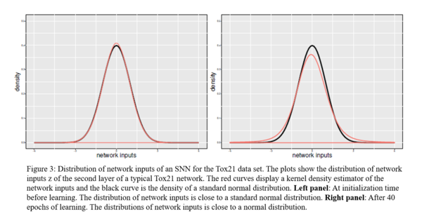
On the Tox21 dataset, the authors demonstrated the self-normalizing effect by comparing the distribution of neural inputs [math]\displaystyle{ z }[/math] at initialization and after 40 epochs of training to that of the standard normal. As Figure 3 show, the distribution of [math]\displaystyle{ z }[/math] remained similar to a normal distribution.
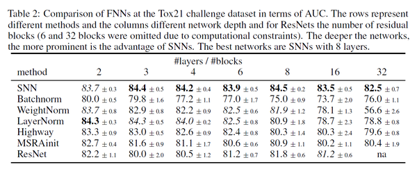
On all three sets of classification tasks, the authors demonstrated that SNN outperformed the other FNN counterparts on accuracy and AUC measures.
SNN achieves close to the state-of-the-art results on the Tox21 dataset with an 8-layer network. The challenge requires prediction of toxic effects of 12000 chemicals based on their chemical structures. SNN with 8 layers had the best performance.
On UCI datasets with fewer than 1,000 observations, SNNs did not outperform SVMs or random forests in terms of average rank in accuracy, but on datasets with at least 1,000 observations, SNNs showed the best overall performance (average rank of 5.8, compared to 6.1 for support vector machines and 6.6 for random forests). Through hyperparameter tuning, it was also discovered that the average depth of FNNs is 10.8 layers, more than the other FNN architectures tried.
In pulsar predictions with the HTRU dataset SNNs produced a new state-of-the-art AUC by a small margin (achieving an AUC 0.98, averaged over 10 cross-validation folds, versus the previous record of 0.976).

Future Work
Although not the focus of this paper, the authors also briefly noted that their initial experiments with applying SELUs on relatively simple CNN structures showed promising results, which is not surprising given that ELUs, which do not have the self-normalizing property, has already been shown to work well with CNNs, demonstrating faster convergence than ReLU networks and even pushing the state-of-the-art error rates on CIFAR-100 at the time of publishing in 2015 [3].
Since the paper was published, SELUs have been adopted by several researchers, not just with FNNs see link, but also with CNNs, GANs, autoencoders, reinforcement learning and RNNs. In a few cases, researchers for those papers concluded that networks trained with SELUs converged faster than those trained with ReLUs, and that SELUs have the same convergence quality as batch normalization. There is potential for SELUs to be incorporated into more architectures in the future.
Critique
Overall, the authors presented a convincing case for using SELUs (along with proper initialization and alpha dropout) on FNNs. FNNs trained with SELU have more layers than those with other normalization techniques, so the work here provides a promising direction for making traditional FNNs more powerful. There are not as many well-established benchmark datasets to evaluate FNNs, but the experiments carried out, particularly on the larger Tox21 dataset, showed that SNNs can be very effective at classification tasks.
The proofs provide a satisfactory explanation for why SELUs have a self-normalising property within the specified domain, but during their introduction the authors give 4 criteria that an activation function must satisfy in order to be self-normalising. Those criteria make intuitive sense, but there is a lack of firm justification which creates some confusion. For example, they state that SNNs cannot be derived from tanh units, even though [math]\displaystyle{ tanh(\lambda x) }[/math] satisfies all 4 criteria if [math]\displaystyle{ \lambda }[/math] is larger than 1. Assuming the authors did not overlook such a simple modification, there must be some additional criteria for an activation function to have a self-normalising property.
The only question I have with the proofs is the lack of explanation for how the domains, [math]\displaystyle{ \Omega }[/math], [math]\displaystyle{ \Omega^- }[/math] and [math]\displaystyle{ \Omega^+ }[/math] are determined, which is an important consideration because they are used for deriving the upper and lower bounds on expressions needed for proving the three theorems. The ranges appear somewhat set through trial-and-error and heuristics to ensure the numbers work out (e.g. make the spectral norm [12] of [math]\displaystyle{ \mathcal{J} }[/math] as large as can be below 1 so as to ensure [math]\displaystyle{ g }[/math] is a contraction mapping), so it is not clear whether they are unique conditions, or that the parameters will remain within those prespecified ranges throughout training; and if the parameters can stray away from the ranges provided, then the issue of what will happen to the self-normalizing property was not addressed. Perhaps that is why the authors gave preference to models with a deeper structure and smaller learning rate during experiments to help the parameters stay within their domains. Further, in addition to the hyperparameters considered, it would be helpful to know the final values that went into the best-performing models, for a better understanding of what range of values work better for SNNs empirically.
Conclusion
The SNN structure proposed in this paper is built on the traditional FNN structure with a few modifications, including the use of SELUs as the activation function (with [math]\displaystyle{ \lambda \approx 1.0507 }[/math] and [math]\displaystyle{ \alpha \approx 1.6733 }[/math]), alpha dropout, network weights initialized with mean of zero and variance [math]\displaystyle{ \frac{1}{n} }[/math], and inputs normalized to mean of zero and variance of one. It is simple to implement while being backed up by detailed theory.
When properly initialized, SELUs will draw neural inputs towards a fixed point of zero mean and unit variance as the activations are propagated through the layers. The self-normalizing property is maintained even when weights deviate from their initial values during training (under mild conditions). When the variance of inputs goes beyond the prespecified range imposed, they are still bounded above and below so SNNs do not suffer from exploding and vanishing gradients. This self-normalizing property allows SNNs to be more robust to perturbations in stochastic gradient descent, so deeper structures with better prediction performance can be built.
In the experiments conducted, the authors demonstrated that SNNs outperformed FNNs trained with other normalization techniques, such as batch, layer and weight normalization, and specialized architectures, such as highway or residual networks, on several classification tasks, including on the UCI Machine Learning Repository datasets. SELUs help in reducing the computation time for normalizing the network relative to RELU+BN and hence is promising. The adoption of SELUs by other researchers also lends credence to the potential for SELUs to be implemented in more neural network architectures.
References
- Ba, Kiros and Hinton. "Layer Normalization". arXiv:1607.06450. (2016).
- Blinn. "Consider the Lowly 2X2 Matrix." IEEE Computer Graphics and Applications. (1996).
- Clevert, Unterthiner, Hochreiter. "Fast and Accurate Deep Network Learning by Exponential Linear Units (ELUs)." arXiv: 1511.07289. (2015).
- He, Zhang, Ren and Sun. "Deep Residual Learning for Image Recognition." arXiv:1512.03385. (2015).
- He, Zhang, Ren and Sun. "Delving Deep into Rectifiers: Surpassing Human-Level Performance on ImageNet Classification." arXiv:1502.01852. (2015).
- Ioffe and Szegedy. "Batch Normalization: Accelerating Deep Network Training by Reducing Internal Covariance Shift." arXiv:1502.03167. (2015).
- Klambauer, Unterthiner, Mayr and Hochreiter. "Self-Normalizing Neural Networks." arXiv: 1706.02515. (2017).
- Salimans and Kingma. "Weight Normalization: A Simple Reparameterization to Accelerate Training of Deep Neural Networks." arXiv:1602.07868. (2016).
- Srivastava, Greff and Schmidhuber. "Highway Networks." arXiv:1505.00387 (2015).
- Unterthiner, Mayr, Klambauer and Hochreiter. "Toxicity Prediction Using Deep Learning." arXiv:1503.01445. (2015).
- https://en.wikipedia.org/wiki/Central_limit_theorem
- http://mathworld.wolfram.com/SpectralNorm.html
- https://www.math.umd.edu/~petersd/466/fixedpoint.pdf
Online Resources
https://github.com/bioinf-jku/SNNs (GitHub repository maintained by some of the paper's authors)
Footnotes
1. Error propagation analysis: The authors performed an error analysis to quantify the potential numerical imprecisions propagated through the numerous operations performed. The potential imprecision [math]\displaystyle{ \epsilon }[/math] was quantified by applying the mean value theorem
\[ |f(x + \Delta x - f(x)| \leqslant ||\triangledown f(x + t\Delta x|| ||\Delta x|| \textrm{ for } t \in [0, 1]\textrm{.} \]
The error propagation rules, or [math]\displaystyle{ |f(x + \Delta x - f(x)| }[/math], was first obtained for simple operations such as addition, subtraction, multiplication, division, square root, exponential function, error function and complementary error function. Them, the error bounds on the compound terms making up [math]\displaystyle{ \Delta (S(\mu, \omega, \nu, \tau, \lambda, \alpha) }[/math] were found by decomposing them into the simpler expressions. If each of the variables have a precision of [math]\displaystyle{ \epsilon }[/math], then it turns out [math]\displaystyle{ S }[/math] has a precision better than [math]\displaystyle{ 292\epsilon }[/math]. For a machine with a precision of [math]\displaystyle{ 2^{-56} }[/math], the rounding error is [math]\displaystyle{ \epsilon \approx 10^{-16} }[/math], and [math]\displaystyle{ 292\epsilon \lt 10^{-13} }[/math]. In addition, all computations are correct up to 3 ulps (“unit in last place”) for the hardware architectures and GNU C library used, with 1 ulp being the highest precision that can be achieved.
2. Independence Assumption: The classic definition of central limit theorem requires [math]\displaystyle{ x_i }[/math]’s to be independent and identically distributed, which is not guaranteed to hold true in a neural network layer. However, according to the Lyapunov CLT, the [math]\displaystyle{ x_i }[/math]’s do not need to be identically distributed as long as the [math]\displaystyle{ (2 + \delta) }[/math]th moment exists for the variables and meet the Lyapunov condition for the rate of growth of the sum of the moments [11]. In addition, CLT has also shown to be valid under weak dependence under mixing conditions [11]. Therefore, the authors argue that the central limit theorem can be applied with network inputs.
3. [math]\displaystyle{ \mathcal{H} }[/math] versus [math]\displaystyle{ \mathcal{J} }[/math] Jacobians: In solving for the largest singular value of the Jacobian [math]\displaystyle{ \mathcal{H} }[/math] for the mapping [math]\displaystyle{ g: (\mu, \nu) }[/math], the authors first worked with the terms in the Jacobian [math]\displaystyle{ \mathcal{J} }[/math] for the mapping [math]\displaystyle{ h: (\mu, \nu) \rightarrow (\widetilde{\mu}, \widetilde{\xi}) }[/math] instead, because the influence of [math]\displaystyle{ \widetilde{\mu} }[/math] on [math]\displaystyle{ \widetilde{\nu} }[/math] is small when [math]\displaystyle{ \widetilde{\mu} }[/math] is small in [math]\displaystyle{ \Omega }[/math] and [math]\displaystyle{ \mathcal{H} }[/math] can be easily expressed as terms in [math]\displaystyle{ \mathcal{J} }[/math]. [math]\displaystyle{ \mathcal{J} }[/math] was referenced in the paper, but I used [math]\displaystyle{ \mathcal{H} }[/math] in the summary here to avoid confusion.
