stat340s13
If you use ideas, plots, text, code and other intellectual property developed by someone else in your `wikicoursenote' contribution , you have to cite the original source. If you copy a sentence or a paragraph from work done by someone else, in addition to citing the original source you have to use quotation marks to identify the scope of the copied material. Evidence of copying or plagiarism will cause a failing mark in the course.
Example of citing the original source
Assumptions Underlying Principal Component Analysis can be found here<ref>http://support.sas.com/publishing/pubcat/chaps/55129.pdf</ref>
Important Notes
To make distinction between the material covered in class and additional material that you have add to the course, use the following convention. For anything that is not covered in the lecture write:
In the news recently was a story that captures some of the ideas behind PCA. Over the past two years, Scott Golder and Michael Macy, researchers from Cornell University, collected 509 million Twitter messages from 2.4 million users in 84 different countries. The data they used were words collected at various times of day and they classified the data into two different categories: positive emotion words and negative emotion words. Then, they were able to study this new data to evaluate subjects' moods at different times of day, while the subjects were in different parts of the world. They found that the subjects generally exhibited positive emotions in the mornings and late evenings, and negative emotions mid-day. They were able to "project their data onto a smaller dimensional space" using PCS. Their paper, "Diurnal and Seasonal Mood Vary with Work, Sleep, and Daylength Across Diverse Cultures," is available in the journal Science.<ref>http://www.pcworld.com/article/240831/twitter_analysis_reveals_global_human_moodiness.html</ref>.
Assumptions Underlying Principal Component Analysis can be found here<ref>http://support.sas.com/publishing/pubcat/chaps/55129.pdf</ref>
Introduction, Class 1 - Tuesday, May 7
Course Instructor: Ali Ghodsi
Lecture:
001: T/Th 8:30-9:50am MC1085
002: T/Th 1:00-2:20pm DC1351
Tutorial:
2:30-3:20pm Mon M3 1006
Office Hours:
Friday at 10am, M3 4208
Midterm
Monday June 17,2013 from 2:30pm-3:20pm
Final
Saturday August 10,2013 from 7:30pm-10:00pm
TA(s):
| TA | Day | Time | Location |
|---|---|---|---|
| Lu Cheng | Monday | 3:30-5:30 pm | M3 3108, space 2 |
| Han ShengSun | Tuesday | 4:00-6:00 pm | M3 3108, space 2 |
| Yizhou Fang | Wednesday | 1:00-3:00 pm | M3 3108, space 1 |
| Huan Cheng | Thursday | 3:00-5:00 pm | M3 3111, space 1 |
| Wu Lin | Friday | 11:00-1:00 pm | M3 3108, space 1 |
Four Fundamental Problems
1 Classification: Given input object X, we have a function which will take this input X and identify which 'class (Y)' it belongs to (Discrete Case)
i.e taking value from x, we could predict y.
(For example, if you have 40 images of oranges and 60 images of apples (represented by x), you can estimate a function that takes the images and states what type of fruit it is - note Y is discrete in this case.)
2 Regression: Same as classification but in the continuous case except y is non discrete. Results from regression are often used for prediction,forecasting and etc. (Example of stock prices, height, weight, etc.)
(A simple practice might be investigating the hypothesis that higher levels of education cause higher levels of income.)
3 Clustering: Use common features of objects in same class or group to form clusters.(in this case, x is given, y is unknown; For example, clustering by provinces to measure average height of Canadian men.)
4 Dimensionality Reduction (also known as Feature extraction, Manifold learning): Used when we have a variable in high dimension space and we want to reduce the dimension
Applications
Most useful when structure of the task is not well understood but can be characterized by a dataset with strong statistical regularity
Examples:
- Computer Vision, Computer Graphics, Finance (fraud detection), Machine Learning
- Search and recommendation (eg. Google, Amazon)
- Automatic speech recognition, speaker verification
- Text parsing
- Face identification
- Tracking objects in video
- Financial prediction(e.g. credit cards)
- Fraud detection
- Medical diagnosis
Course Information
Prerequisite: (One of CS 116, 126/124, 134, 136, 138, 145, SYDE 221/322) and (STAT 230 with a grade of at least 60% or STAT 240) and (STAT 231 or 241)
Antirequisite: CM 361/STAT 341, CS 437, 457
General Information
- No required textbook
- Recommended: "Simulation" by Sheldon M. Ross
- Computing parts of the course will be done in Matlab, but prior knowledge of Matlab is not essential (will have a tutorial on it)
- First midterm will be held on Monday, June 17 from 2:30 to 3:30
- Announcements and assignments will be posted on Learn.
- Other course material on: http://wikicoursenote.com/wiki/
- Log on to both Learn and wikicoursenote frequently.
- Email all questions and concerns to UWStat340@gmail.com. Do not use your personal email address! Do not email instructor or TAs about the class directly to their personal accounts!
Wikicourse note (complete at least 12 contributions to get 10% of final mark):
When applying for an account in the wikicourse note, please use the quest account as your login name while the uwaterloo email as the registered email. This is important as the quest id will be used to identify the students who make the contributions.
Example:
User: questid
Email: questid@uwaterloo.ca
After the student has made the account request, do wait for several hours before students can login into the account using the passwords stated in the email. During the first login, students will be ask to create a new password for their account.
As a technical/editorial contributor: Make contributions within 1 week and do not copy the notes on the blackboard.
All contributions are now considered general contributions you must contribute to 50% of lectures for full marks
- A general contribution can be correctional (fixing mistakes) or technical (expanding content, adding examples, etc.) but at least half of your contributions should be technical for full marks.
Do not submit copyrighted work without permission, cite original sources. Each time you make a contribution, check mark the table. Marks are calculated on an honour system, although there will be random verifications. If you are caught claiming to contribute but have not, you will not be credited.
Wikicoursenote contribution form : https://docs.google.com/forms/d/1Sgq0uDztDvtcS5JoBMtWziwH96DrBz2JiURvHPNd-xs/viewform
- you can submit your contributions multiple times.
- you will be able to edit the response right after submitting
- send email to make changes to an old response : uwstat340@gmail.com
Tentative Topics
- Random variable and stochastic process generation
- Discrete-Event Systems
- Variance reduction
- Markov Chain Monte Carlo
Class 2 - Thursday, May 9
Generating Random Numbers
Introduction
Simulation is the imitation of a process or system over time. Computational power has introduced the possibility of using simulation study to analyze models used to describe a situation.
In order to perform a simulation study, we should:
<br\> 1 Use a computer to generate (pseudo*) random numbers (rand in MATLAB).
2 Use these numbers to generate values of random variable from distributions: for example, set a variable in terms of uniform u ~ U(0,1).
3 Using the concept of discrete events, we show how the random variables can be used to generate the behavior of a stochastic model over time. (Note: A stochastic model is the opposite of deterministic model, where there are several directions the process can evolve to)
4 After continually generating the behavior of the system, we can obtain estimators and other quantities of interest.
The building block of a simulation study is the ability to generate a random number. This random number is a value from a random variable distributed uniformly on (0,1). There are many different methods of generating a random number:
Physical Method: Roulette wheel, lottery balls, dice rolling, card shuffling etc.


Numerically/Arithmetically: Use of a computer to successively generate pseudorandom numbers. The
sequence of numbers can appear to be random; however they are deterministically calculated with an
equation which defines pseudorandom.
(Source: Ross, Sheldon M., and Sheldon M. Ross. Simulation. San Diego: Academic, 1997. Print.)
- We use the prefix pseudo because computer generates random numbers based on algorithms, which suggests that generated numbers are not truly random. Therefore pseudo-random numbers is used.
In general, a deterministic model produces specific results given certain inputs by the model user, contrasting with a stochastic model which encapsulates randomness and probabilistic events.

A computer cannot generate truly random numbers because computers can only run algorithms, which are deterministic in nature. They can, however, generate Pseudo Random Numbers
Pseudo Random Numbers are the numbers that seem random but are actually determined by a relative set of original values. It is a chain of numbers pre-set by a formula or an algorithm, and the value jump from one to the next, making it look like a series of independent random events. The flaw of this method is that, eventually the chain returns to its initial position and pattern starts to repeat, but if we make the number set large enough we can prevent the numbers from repeating too early. Although the pseudo random numbers are deterministic, these numbers have a sequence of value and all of them have the appearances of being independent uniform random variables. Being deterministic, pseudo random numbers are valuable and beneficial due to the ease to generate and manipulate.
When people repeat the test many times, the results will be the closed express values, which make the trials look deterministic. However, for each trial, the result is random. So, it looks like pseudo random numbers.
Mod
Let [math]\displaystyle{ n \in \N }[/math] and [math]\displaystyle{ m \in \N^+ }[/math], then by Division Algorithm,
[math]\displaystyle{ \exists q, \, r \in \N \;\text{with}\; 0\leq r \lt m, \; \text{s.t.}\; n = mq+r }[/math],
where [math]\displaystyle{ q }[/math] is called the quotient and [math]\displaystyle{ r }[/math] the remainder. Hence we can define a binary function
[math]\displaystyle{ \mod : \N \times \N^+ \rightarrow \N }[/math] given by [math]\displaystyle{ r:=n \mod m }[/math] which returns the remainder after division by m.
Generally, mod means taking the reminder after division by m.
We say that n is congruent to r mod m if n = mq + r, where m is an integer.
Values are between 0 and m-1
if y = ax + b, then [math]\displaystyle{ b:=y \mod a }[/math].
Example 1:
[math]\displaystyle{ 30 = 4 \cdot 7 + 2 }[/math]
[math]\displaystyle{ 2 := 30\mod 7 }[/math]
[math]\displaystyle{ 25 = 8 \cdot 3 + 1 }[/math]
[math]\displaystyle{ 1: = 25\mod 3 }[/math]
[math]\displaystyle{ -3=5\cdot (-1)+2 }[/math]
[math]\displaystyle{ 2:=-3\mod 5 }[/math]
Example 2:
If [math]\displaystyle{ 23 = 3 \cdot 6 + 5 }[/math]
Then equivalently, [math]\displaystyle{ 5 := 23\mod 6 }[/math]
If [math]\displaystyle{ 31 = 31 \cdot 1 }[/math]
Then equivalently, [math]\displaystyle{ 0 := 31\mod 31 }[/math]
If [math]\displaystyle{ -37 = 40\cdot (-1)+ 3 }[/math]
Then equivalently, [math]\displaystyle{ 3 := -37\mod 40 }[/math]
Example 3:
[math]\displaystyle{ 77 = 3 \cdot 25 + 2 }[/math]
[math]\displaystyle{ 2 := 77\mod 3 }[/math]
[math]\displaystyle{ 25 = 25 \cdot 1 + 0 }[/math]
[math]\displaystyle{ 0: = 25\mod 25 }[/math]
Note: [math]\displaystyle{ \mod }[/math] here is different from the modulo congruence relation in [math]\displaystyle{ \Z_m }[/math], which is an equivalence relation instead of a function.
The modulo operation is useful for determining if an integer divided by another integer produces a non-zero remainder. But both integers should satisfy [math]\displaystyle{ n = mq + r }[/math], where [math]\displaystyle{ m }[/math], [math]\displaystyle{ r }[/math], [math]\displaystyle{ q }[/math], and [math]\displaystyle{ n }[/math] are all integers, and [math]\displaystyle{ r }[/math] is smaller than [math]\displaystyle{ m }[/math]. The above rules also satisfy when any of [math]\displaystyle{ m }[/math], [math]\displaystyle{ r }[/math], [math]\displaystyle{ q }[/math], and [math]\displaystyle{ n }[/math] is negative integer, see the third example.
Mixed Congruential Algorithm
We define the Linear Congruential Method to be [math]\displaystyle{ x_{k+1}=(ax_k + b) \mod m }[/math], where [math]\displaystyle{ x_k, a, b, m \in \N, \;\text{with}\; a, m \neq 0 }[/math]. Given a seed (i.e. an initial value [math]\displaystyle{ x_0 \in \N }[/math]), we can obtain values for [math]\displaystyle{ x_1, \, x_2, \, \cdots, x_n }[/math] inductively. The Multiplicative Congruential Method, invented by Berkeley professor D. H. Lehmer, may also refer to the special case where [math]\displaystyle{ b=0 }[/math] and the Mixed Congruential Method is case where [math]\displaystyle{ b \neq 0 }[/math]
. Their title as "mixed" arises from the fact that it has both a multiplicative and additive term.
An interesting fact about Linear Congruential Method is that it is one of the oldest and best-known pseudo random number generator algorithms. It is very fast and requires minimal memory to retain state. However, this method should not be used for applications that require high randomness. They should not be used for Monte Carlo simulation and cryptographic applications. (Monte Carlo simulation will consider possibilities for every choice of consideration, and it shows the extreme possibilities. This method is not precise enough.)
 "Source: STAT 340 Spring 2010 Course Notes"
First consider the following algorithm
[math]\displaystyle{ x_{k+1}=x_{k} \mod m }[/math]
such that: if [math]\displaystyle{ x_{0}=5(mod 150) }[/math], [math]\displaystyle{ x_{n}=3x_{n-1} }[/math], find [math]\displaystyle{ x_{1},x_{8},x_{9} }[/math].
[math]\displaystyle{ x_{n}=(3^n)*5(mod 150) }[/math]
[math]\displaystyle{ x_{1}=45,x_{8}=105,x_{9}=15 }[/math]
Example
[math]\displaystyle{ \text{Let }x_{0}=10,\,m=3 }[/math]
- [math]\displaystyle{ \begin{align} x_{1} &{}= 10 &{}\mod{3} = 1 \\ x_{2} &{}= 1 &{}\mod{3} = 1 \\ x_{3} &{}= 1 &{}\mod{3} =1 \\ \end{align} }[/math]
[math]\displaystyle{ \ldots }[/math]
Excluding [math]\displaystyle{ x_{0} }[/math], this example generates a series of ones. In general, excluding [math]\displaystyle{ x_{0} }[/math], the algorithm above will always generate a series of the same number less than M. Hence, it has a period of 1. The period can be described as the length of a sequence before it repeats. We want a large period with a sequence that is random looking. We can modify this algorithm to form the Multiplicative Congruential Algorithm.
[math]\displaystyle{ x_{k+1}=(a \cdot x_{k} + b) \mod m }[/math](a little tip: [math]\displaystyle{ (a \cdot b)\mod c = (a\mod c)\cdot(b\mod c)) }[/math]
Example
[math]\displaystyle{ \text{Let }a=2,\, b=1, \, m=3, \, x_{0} = 10 }[/math]
[math]\displaystyle{ \begin{align}
\text{Step 1: } 0&{}=(2\cdot 10 + 1) &{}\mod 3 \\
\text{Step 2: } 1&{}=(2\cdot 0 + 1) &{}\mod 3 \\
\text{Step 3: } 0&{}=(2\cdot 1 + 1) &{}\mod 3 \\
\end{align} }[/math]
[math]\displaystyle{ \ldots }[/math]
This example generates a sequence with a repeating cycle of two integers.
(If we choose the numbers properly, we could get a sequence of "random" numbers. How do we find the value of [math]\displaystyle{ a,b, }[/math] and [math]\displaystyle{ m }[/math]? At the very least [math]\displaystyle{ m }[/math] should be a very large, preferably prime number. The larger [math]\displaystyle{ m }[/math] is, the higher the possibility to get a sequence of "random" numbers. This is easier to solve in Matlab. In Matlab, the command rand() generates random numbers which are uniformly distributed on the interval (0,1)). Matlab uses [math]\displaystyle{ a=7^5, b=0, m=2^{31}-1 }[/math] – recommended in a 1988 paper, "Random Number Generators: Good Ones Are Hard To Find" by Stephen K. Park and Keith W. Miller (Important part is that [math]\displaystyle{ m }[/math] should be large and prime)
Note: [math]\displaystyle{ \frac {x_{n+1}}{m-1} }[/math] is an approximation to the value of a U(0,1) random variable.
MatLab Instruction for Multiplicative Congruential Algorithm:
Before you start, you need to clear all existing defined variables and operations:
>>clear all
>>close all
>>a=17
>>b=3
>>m=31
>>x=5
>>mod(a*x+b,m)
ans=26
>>x=mod(a*x+b,m)
(Note:
1. Keep repeating this command over and over again and you will get random numbers – this is how the command rand works in a computer.
2. There is a function in MATLAB called RAND to generate a random number between 0 and 1.
For example, in MATLAB, we can use rand(1,1000) to generate 1000's numbers between 0 and 1. This is essentially a vector with 1 row, 1000 columns, with each entry a random number between 0 and 1.
3. If we would like to generate 1000 or more numbers, we could use a for loop
(Note on MATLAB commands:
1. clear all: clears all variables.
2. close all: closes all figures.
3. who: displays all defined variables.
4. clc: clears screen.
5. ; : prevents the results from printing.
6. disstool: displays a graphing tool.
>>a=13
>>b=0
>>m=31
>>x(1)=1
>>for ii=2:1000
x(ii)=mod(a*x(ii-1)+b,m);
end
>>size(x)
ans=1    1000
>>hist(x)

(Note: The semicolon after the x(ii)=mod(a*x(ii-1)+b,m) ensures that Matlab will not print the entire vector of x. It will instead calculate it internally and you will be able to work with it. Adding the semicolon to the end of this line reduces the run time significantly.)
This algorithm involves three integer parameters [math]\displaystyle{ a, b, }[/math] and [math]\displaystyle{ m }[/math] and an initial value, [math]\displaystyle{ x_0 }[/math] called the seed. A sequence of numbers is defined by [math]\displaystyle{ x_{k+1} = ax_k+ b \mod m }[/math].
Note: For some bad [math]\displaystyle{ a }[/math] and [math]\displaystyle{ b }[/math], the histogram may not look uniformly distributed.
Note: In MATLAB, hist(x) will generate a graph representing the distribution. Use this function after you run the code to check the real sample distribution.
Example: [math]\displaystyle{ a=13, b=0, m=31 }[/math]
The first 30 numbers in the sequence are a permutation of integers from 1 to 30, and then the sequence repeats itself so it is important to choose [math]\displaystyle{ m }[/math] large to decrease the probability of each number repeating itself too early. Values are between [math]\displaystyle{ 0 }[/math] and [math]\displaystyle{ m-1 }[/math]. If the values are normalized by dividing by [math]\displaystyle{ m-1 }[/math], then the results are approximately numbers uniformly distributed in the interval [0,1]. There is only a finite number of values (30 possible values in this case). In MATLAB, you can use function "hist(x)" to see if it looks uniformly distributed. We saw that the values between 0-30 had the same frequency in the histogram, so we can conclude that they are uniformly distributed.
If [math]\displaystyle{ x_0=1 }[/math], then
- [math]\displaystyle{ x_{k+1} = 13x_{k}\mod{31} }[/math]
So,
- [math]\displaystyle{ \begin{align} x_{0} &{}= 1 \\ x_{1} &{}= 13 \times 1 + 0 &{}\mod{31} = 13 \\ x_{2} &{}= 13 \times 13 + 0 &{}\mod{31} = 14 \\ x_{3} &{}= 13 \times 14 + 0 &{}\mod{31} =27 \\ \end{align} }[/math]
etc.
For example, with [math]\displaystyle{ a = 3, b = 2, m = 4, x_0 = 1 }[/math], we have:
- [math]\displaystyle{ x_{k+1} = (3x_{k} + 2)\mod{4} }[/math]
So,
- [math]\displaystyle{ \begin{align}
x_{0} &{}= 1 \\
x_{1} &{}= 3 \times 1 + 2 \mod{4} = 1 \\
x_{2} &{}= 3 \times 1 + 2 \mod{4} = 1 \\
\end{align} }[/math]
Another Example, a =3, b =2, m = 5, x_0=1 etc.
FAQ:
1.Why is it 1 to 30 instead of 0 to 30 in the example above?
[math]\displaystyle{ b = 0 }[/math] so in order to have [math]\displaystyle{ x_k }[/math] equal to 0, [math]\displaystyle{ x_{k-1} }[/math] must be 0 (since [math]\displaystyle{ a=13 }[/math] is relatively prime to 31). However, the seed is 1. Hence, we will never observe 0 in the sequence.
Alternatively, {0} and {1,2,...,30} are two orbits of the left multiplication by 13 in the group [math]\displaystyle{ \Z_{31} }[/math].
2.Will the number 31 ever appear?Is there a probability that a number never appears?
The number 31 will never appear. When you perform the operation [math]\displaystyle{ \mod m }[/math], the largest possible answer that you could receive is [math]\displaystyle{ m-1 }[/math]. Whether or not a particular number in the range from 0 to [math]\displaystyle{ m - 1 }[/math] appears in the above algorithm will be dependent on the values chosen for [math]\displaystyle{ a, b }[/math] and [math]\displaystyle{ m }[/math].
Examples:[From Textbook]
[math]\displaystyle{ \text{If }x_0=3 \text{ and } x_n=(5x_{n-1}+7)\mod 200 }[/math], [math]\displaystyle{ \text{find }x_1,\cdots,x_{10} }[/math].
Solution:
[math]\displaystyle{ \begin{align}
x_1 &{}= (5 \times 3+7) &{}\mod{200} &{}= 22 \\
x_2 &{}= 117 &{}\mod{200} &{}= 117 \\
x_3 &{}= 592 &{}\mod{200} &{}= 192 \\
x_4 &{}= 2967 &{}\mod{200} &{}= 167 \\
x_5 &{}= 14842 &{}\mod{200} &{}= 42 \\
x_6 &{}= 74217 &{}\mod{200} &{}= 17 \\
x_7 &{}= 371092 &{}\mod{200} &{}= 92 \\
x_8 &{}= 1855467 &{}\mod{200} &{}= 67 \\
x_9 &{}= 9277342 &{}\mod{200} &{}= 142 \\
x_{10} &{}= 46386717 &{}\mod{200} &{}= 117 \\
\end{align} }[/math]
Comments:
Matlab code: a=5; b=7; m=200; x(1)=3; for ii=2:1000 x(ii)=mod(a*x(ii-1)+b,m); end size(x); hist(x)
Typically, it is good to choose [math]\displaystyle{ m }[/math] such that [math]\displaystyle{ m }[/math] is large, and [math]\displaystyle{ m }[/math] is prime. Careful selection of parameters '[math]\displaystyle{ a }[/math]' and '[math]\displaystyle{ b }[/math]' also helps generate relatively "random" output values, where it is harder to identify patterns. For example, when we used a composite (non prime) number such as 40 for [math]\displaystyle{ m }[/math], our results were not satisfactory in producing an output resembling a uniform distribution.
The computed values are between 0 and [math]\displaystyle{ m-1 }[/math]. If the values are normalized by dividing by [math]\displaystyle{ m-1 }[/math], their result is numbers uniformly distributed on the interval [math]\displaystyle{ \left[0,1\right] }[/math] (similar to computing from uniform distribution).
From the example shown above, if we want to create a large group of random numbers, it is better to have large, prime [math]\displaystyle{ m }[/math] so that the generated random values will not repeat after several iterations. Note: the period for this example is 8: from '[math]\displaystyle{ x_2 }[/math]' to '[math]\displaystyle{ x_9 }[/math]'.
There has been a research on how to choose uniform sequence. Many programs give you the options to choose the seed. Sometimes the seed is chosen by CPU.
Theorem (extra knowledge)
Let c be a non-zero constant. Then for any seed x0, and LCG will have largest max. period if and only if
(i) m and c are coprime;
(ii) (a-1) is divisible by all prime factor of m;
(iii) if and only if m is divisible by 4, then a-1 is also divisible by 4.
We want our LCG to have a large cycle. We call a cycle with m element the maximal period. We can make it bigger by making m big and prime. Recall:any number you can think of can be broken into a factor of prime Define coprime:Two numbers X and Y, are coprime if they do not share any prime factors.
Example:
Xn=(15Xn-1 + 4) mod 7
(i) m=7 c=4 -> coprime;
(ii) a-1=14 and a-1 is divisible by 7;
(iii) dose not apply.
(The extra knowledge stops here)
In this part, I learned how to use R code to figure out the relationship between two integers division, and their remainder. And when we use R to calculate R with random variables for a range such as(1:1000),the graph of distribution is like uniform distribution.
Summary of Multiplicative Congruential Algorithm
Problem: generate Pseudo Random Numbers.
Plan:
- find integer: a b m(large prime) x0(the seed) .
- [math]\displaystyle{ x_{k+1}=(ax_{k}+b) }[/math]mod m
Matlab Instruction:
>>clear all
>>close all
>>a=17
>>b=3
>>m=31
>>x=5
>>mod(a*x+b,m)
ans=26
>>x=mod(a*x+b,m)
Another algorithm for generating pseudo random numbers is the multiply with carry method. Its simplest form is similar to the linear congruential generator. They differs in that the parameter b changes in the MWC algorithm. It is as follows:
1.) xk+1 = axk + bk mod m
2.) bk+1 = floor((axk + bk)/m)
3.) set k to k + 1 and go to step 1
Inverse Transform Method
Now that we know how to generate random numbers, we use these values to sample form distributions such as exponential. However, to easily use this method, the probability distribution consumed must have a cumulative distribution function (cdf) [math]\displaystyle{ F }[/math] with a tractable (that is, easily found) inverse [math]\displaystyle{ F^{-1} }[/math].
Theorem:
If we want to generate the value of a discrete random variable X, we must generate a random number U, uniformly distributed over (0,1).
Let [math]\displaystyle{ F:\R \rightarrow \left[0,1\right] }[/math] be a cdf. If [math]\displaystyle{ U \sim U\left[0,1\right] }[/math], then the random variable given by [math]\displaystyle{ X:=F^{-1}\left(U\right) }[/math]
follows the distribution function [math]\displaystyle{ F\left(\cdot\right) }[/math],
where [math]\displaystyle{ F^{-1}\left(u\right):=\inf F^{-1}\big(\left[u,+\infty\right)\big) = \inf\{x\in\R | F\left(x\right) \geq u\} }[/math] is the generalized inverse.
Note: [math]\displaystyle{ F }[/math] need not be invertible everywhere on the real line, but if it is, then the generalized inverse is the same as the inverse in the usual case. We only need it to be invertible on the range of F(x), [0,1].
Proof of the theorem:
The generalized inverse satisfies the following:
- [math]\displaystyle{ P(X\leq x) }[/math]
[math]\displaystyle{ = P(F^{-1}(U)\leq x) }[/math] (since [math]\displaystyle{ X= F^{-1}(U) }[/math] by the inverse method)
[math]\displaystyle{ = P((F(F^{-1}(U))\leq F(x)) }[/math] (since [math]\displaystyle{ F }[/math] is monotonically increasing)
[math]\displaystyle{ = P(U\leq F(x)) }[/math] (since [math]\displaystyle{ P(U\leq a)= a }[/math] for [math]\displaystyle{ U \sim U(0,1), a \in [0,1] }[/math],
[math]\displaystyle{ = F(x) , \text{ where } 0 \leq F(x) \leq 1 }[/math]
This is the c.d.f. of X.
That is [math]\displaystyle{ F^{-1}\left(u\right) \leq x \Leftrightarrow u \leq F\left(x\right) }[/math]
Finally, [math]\displaystyle{ P(X \leq x) = P(F^{-1}(U) \leq x) = P(U \leq F(x)) = F(x) }[/math], since [math]\displaystyle{ U }[/math] is uniform on the unit interval.
This completes the proof.
Therefore, in order to generate a random variable X~F, it can generate U according to U(0,1) and then make the transformation x=[math]\displaystyle{ F^{-1}(U) }[/math]
Note that we can apply the inverse on both sides in the proof of the inverse transform only if the pdf of X is monotonic. A monotonic function is one that is either increasing for all x, or decreasing for all x. Of course, this holds true for all CDFs, since they are monotonic by definition.
In short, what the theorem tells us is that we can use a random number [math]\displaystyle{ U from U(0,1) }[/math] to randomly sample a point on the CDF of X, then apply the inverse of the CDF to map the given probability to its domain, which gives us the random variable X.
Example 1 - Exponential: [math]\displaystyle{ f(x) = \lambda e^{-\lambda x} }[/math]
Calculate the CDF:
[math]\displaystyle{ F(x)= \int_0^x f(t) dt = \int_0^x \lambda e ^{-\lambda t}\ dt }[/math]
[math]\displaystyle{ = \frac{\lambda}{-\lambda}\, e^{-\lambda t}\, | \underset{0}{x} }[/math]
[math]\displaystyle{ = -e^{-\lambda x} + e^0 =1 - e^{- \lambda x} }[/math]
Solve the inverse:
[math]\displaystyle{ y=1-e^{- \lambda x} \Rightarrow 1-y=e^{- \lambda x} \Rightarrow x=-\frac {ln(1-y)}{\lambda} }[/math]
[math]\displaystyle{ y=-\frac {ln(1-x)}{\lambda} \Rightarrow F^{-1}(x)=-\frac {ln(1-x)}{\lambda} }[/math]
Note that 1 − U is also uniform on (0, 1) and thus −log(1 − U) has the same distribution as −logU.
Steps:
Step 1: Draw U ~U[0,1];
Step 2: [math]\displaystyle{ x=\frac{-ln(U)}{\lambda} }[/math]
EXAMPLE 2 Normal distribution
G(y)=P[Y<=y)
     =P[-sqr (y) < z < sqr (y))
     =integrate from -sqr(z) to Sqr(z) 1/sqr(2pi) e ^(-z^2/2) dz
     = 2 integrate from 0 to sqr(y)  1/sqr(2pi) e ^(-z^2/2) dz
its the cdf of Y=z^2
pdf g(y)= G'(y) pdf pf x^2 (1)
MatLab Code:
>>u=rand(1,1000);
>>hist(u)       # this will generate a fairly uniform diagram
.jpg)
#let λ=2 in this example; however, you can make another value for λ
>>x=(-log(1-u))/2;
>>size(x)       #1000 in size
>>figure
>>hist(x)       #exponential
.jpg)
Example 2 - Continuous Distribution:
[math]\displaystyle{ f(x) = \dfrac {\lambda } {2}e^{-\lambda \left| x-\theta \right| } for -\infty \lt X \lt \infty , \lambda \gt 0 }[/math]
Calculate the CDF:
[math]\displaystyle{ F(x)= \frac{1}{2} e^{-\lambda (\theta - x)} , for \ x \le \theta }[/math]
[math]\displaystyle{ F(x) = 1 - \frac{1}{2} e^{-\lambda (x - \theta)}, for \ x \gt \theta }[/math]
Solve for the inverse:
[math]\displaystyle{ F^{-1}(x)= \theta + ln(2y)/\lambda, for \ 0 \le y \le 0.5 }[/math]
[math]\displaystyle{ F^{-1}(x)= \theta - ln(2(1-y))/\lambda, for \ 0.5 \lt y \le 1 }[/math]
Algorithm:
Steps:
Step 1: Draw U ~ U[0, 1];
Step 2: Compute [math]\displaystyle{ X = F^-1(U) }[/math] i.e. [math]\displaystyle{ X = \theta + \frac {1}{\lambda} ln(2U) }[/math] for U < 0.5 else [math]\displaystyle{ X = \theta -\frac {1}{\lambda} ln(2(1-U)) }[/math]
Example 3 - [math]\displaystyle{ F(x) = x^5 }[/math]:
Given a CDF of X: [math]\displaystyle{ F(x) = x^5 }[/math], transform U~U[0,1].
Sol:
Let [math]\displaystyle{ y=x^5 }[/math], solve for x: [math]\displaystyle{ x=y^\frac {1}{5} }[/math]. Therefore, [math]\displaystyle{ F^{-1} (x) = x^\frac {1}{5} }[/math]
Hence, to obtain a value of x from F(x), we first set 'u' as an uniform distribution, then obtain the inverse function of F(x), and set
[math]\displaystyle{ x= u^\frac{1}{5} }[/math]
Algorithm:
Steps:
Step 1: Draw U ~ rand[0, 1];
Step 2: X=U^(1/5);
Example 4 - BETA(1,β):
Given u~U[0,1], generate x from BETA(1,β)
Solution:
[math]\displaystyle{ F(x)= 1-(1-x)^\beta }[/math],
[math]\displaystyle{ u= 1-(1-x)^\beta }[/math]
Solve for x:
[math]\displaystyle{ (1-x)^\beta = 1-u }[/math],
[math]\displaystyle{ 1-x = (1-u)^\frac {1}{\beta} }[/math],
[math]\displaystyle{ x = 1-(1-u)^\frac {1}{\beta} }[/math]
let β=3, use Matlab to construct N=1000 observations from Beta(1,3)
MatLab Code:
>> u = rand(1,1000);
x = 1-(1-u)^(1/3);
>> hist(x,50)
>> mean(x)
Example 5 - Estimating [math]\displaystyle{ \pi }[/math]:
Let's use rand() and Monte Carlo Method to estimate [math]\displaystyle{ \pi }[/math]
N= total number of points
Nc = total number of points inside the circle
Prob[(x,y) lies in the circle=[math]\displaystyle{ \frac {Area(circle)}{Area(square)} }[/math]
If we take square of size 2, circle will have area =[math]\displaystyle{ \pi (\frac {2}{2})^2 =\pi }[/math].
Thus [math]\displaystyle{ \pi= 4(\frac {N_c}{N}) }[/math]
  For example, UNIF(a,b)

  [math]\displaystyle{ y = F(x) = (x - a)/ (b - a)  }[/math]
  [math]\displaystyle{ x = (b - a ) * y + a }[/math]
  [math]\displaystyle{ X = a + ( b - a) * U }[/math]

  where U is UNIF(0,1)
Limitations:
1. This method is flawed since not all functions are invertible or monotonic: generalized inverse is hard to work on.
2. It may be impractical since some CDF's and/or integrals are not easy to compute such as Gaussian distribution.
We learned how to prove the transformation from cdf to inverse cdf,and use the uniform distribution to obtain a value of x from F(x). We can also use uniform distribution in inverse method to determine other distributions. The probability of getting a point for a circle over the triangle is a closed uniform distribution, each point in the circle and over the triangle is almost the same. Then, we can look at the graph to determine what kind of distribution the graph resembles.
Probability Distribution Function Tool in MATLAB
disttool #shows different distributions
This command allows users to explore different types of distribution and see how the changes affect the parameters on the plot of either a CDF or PDF.
 change the value of mu and sigma can change the graph skew side.
Class 3 - Tuesday, May 14
Recall the Inverse Transform Method
Let U~Unif(0,1),then the random variable X = F-1(u) has distribution F.
To sample X with CDF F(x),
[math]\displaystyle{ 1) U~ \sim~ Unif [0,1] }[/math]
2) X = F-1(u)
Note: CDF of a U(a,b) random variable is:
- [math]\displaystyle{ F(x)= \begin{cases} 0 & \text{for }x \lt a \\[8pt] \frac{x-a}{b-a} & \text{for }a \le x \lt b \\[8pt] 1 & \text{for }x \ge b \end{cases} }[/math]
Thus, for [math]\displaystyle{ U }[/math] ~ [math]\displaystyle{ U(0,1) }[/math], we have [math]\displaystyle{ P(U\leq 1) = 1 }[/math] and [math]\displaystyle{ P(U\leq 1/2) = 1/2 }[/math].
More generally, we see that [math]\displaystyle{ P(U\leq a) = a }[/math].
For this reason, we had [math]\displaystyle{ P(U\leq F(x)) = F(x) }[/math].
Reminder:
This is only for uniform distribution [math]\displaystyle{ U~ \sim~ Unif [0,1] }[/math]
[math]\displaystyle{ P (U \le 1) = 1 }[/math]
[math]\displaystyle{ P (U \le 0.5) = 0.5 }[/math]
[math]\displaystyle{ P (U \le a) = a }[/math]
 [math]\displaystyle{ P(U\leq a)=a }[/math]
Note that on a single point there is no mass probability (i.e. [math]\displaystyle{ u }[/math] <= 0.5, is the same as [math]\displaystyle{ u }[/math] < 0.5) More formally, this is saying that [math]\displaystyle{ P(X = x) = F(x)- \lim_{s \to x^-}F(x) }[/math] , which equals zero for any continuous random variable
Limitations of the Inverse Transform Method
Though this method is very easy to use and apply, it does have a major disadvantage/limitation:
- We need to find the inverse cdf [math]\displaystyle{ F^{-1}(\cdot) }[/math]. In some cases the inverse function does not exist, or is difficult to find because it requires a closed form expression for F(x).
For example, it is too difficult to find the inverse cdf of the Gaussian distribution, so we must find another method to sample from the Gaussian distribution.
In conclusion, we need to find another way of sampling from more complicated distributions
Discrete Case
The same technique can be used for discrete case. We want to generate a discrete random variable x, that has probability mass function:
- [math]\displaystyle{ \begin{align}P(X = x_i) &{}= p_i \end{align} }[/math]
- [math]\displaystyle{ x_0 \leq x_1 \leq x_2 \dots \leq x_n }[/math]
- [math]\displaystyle{ \sum p_i = 1 }[/math]
Algorithm for applying Inverse Transformation Method in Discrete Case (Procedure):
1. Define a probability mass function for [math]\displaystyle{ x_{i} }[/math] where i = 1,....,k. Note: k could grow infinitely.
2. Generate a uniform random number U, [math]\displaystyle{ U~ \sim~ Unif [0,1] }[/math]
3. If [math]\displaystyle{ U\leq p_{o} }[/math], deliver [math]\displaystyle{ X = x_{o} }[/math]
4. Else, if [math]\displaystyle{ U\leq p_{o} + p_{1} }[/math], deliver [math]\displaystyle{ X = x_{1} }[/math]
5. Repeat the process again till we reached to [math]\displaystyle{ U\leq p_{o} + p_{1} + ......+ p_{k} }[/math], deliver [math]\displaystyle{ X = x_{k} }[/math]
Note that after generating a random U, the value of X can be determined by finding the interval [math]\displaystyle{ [F(x_{j-1}),F(x_{j})] }[/math] in which U lies.
Example 3.0:
Generate a random variable from the following probability function:
| x | -2 | -1 | 0 | 1 | 2 |
| f(x) | 0.1 | 0.5 | 0.07 | 0.03 | 0.3 |
Answer:
1. Gen U~U(0,1)
2. If U < 0.5 then output -1
else if U < 0.8 then output 2
else if U < 0.9 then output -2
else if U < 0.97 then output 0 else output 1
Example 3.1 (from class): (Coin Flipping Example)
We want to simulate a coin flip. We have U~U(0,1) and X = 0 or X = 1.
We can define the U function so that:
If [math]\displaystyle{ U\leq 0.5 }[/math], then X = 0
and if [math]\displaystyle{ 0.5 \lt U\leq 1 }[/math], then X =1.
This allows the probability of Heads occurring to be 0.5 and is a good generator of a random coin flip.
[math]\displaystyle{ U~ \sim~ Unif [0,1] }[/math]
- [math]\displaystyle{ \begin{align} P(X = 0) &{}= 0.5\\ P(X = 1) &{}= 0.5\\ \end{align} }[/math]
The answer is:
- [math]\displaystyle{ x = \begin{cases} 0, & \text{if } U\leq 0.5 \\ 1, & \text{if } 0.5 \lt U \leq 1 \end{cases} }[/math]
- Code
>>for ii=1:1000
    u=rand;
      if u<0.5
         x(ii)=0;
      else
         x(ii)=1;
      end
  end
>>hist(x)

Note: The role of semi-colon in Matlab: Matlab will not print out the results if the line ends in a semi-colon and vice versa.
Example 3.2 (From class):
Suppose we have the following discrete distribution:
- [math]\displaystyle{ \begin{align} P(X = 0) &{}= 0.3 \\ P(X = 1) &{}= 0.2 \\ P(X = 2) &{}= 0.5 \end{align} }[/math]

The cumulative distribution function (cdf) for this distribution is then:
- [math]\displaystyle{ F(x) = \begin{cases} 0, & \text{if } x \lt 0 \\ 0.3, & \text{if } x \lt 1 \\ 0.5, & \text{if } x \lt 2 \\ 1, & \text{if } x \ge 2 \end{cases} }[/math]
Then we can generate numbers from this distribution like this, given [math]\displaystyle{ U \sim~ Unif[0, 1] }[/math]:
- [math]\displaystyle{ x = \begin{cases} 0, & \text{if } U\leq 0.3 \\ 1, & \text{if } 0.3 \lt U \leq 0.5 \\ 2, & \text{if } 0.5 \lt U\leq 1 \end{cases} }[/math]
"Procedure"
1. Draw U~u (0,1)
2. if U<=0.3 deliver x=0
3. else if 0.3<U<=0.5 deliver x=1
4. else 0.5<U<=1 deliver x=2
Can you find a faster way to run this algorithm? Consider:
- [math]\displaystyle{ x = \begin{cases} 2, & \text{if } U\leq 0.5 \\ 1, & \text{if } 0.5 \lt U \leq 0.7 \\ 0, & \text{if } 0.7 \lt U\leq 1 \end{cases} }[/math]
The logic for this is that U is most likely to fall into the largest range. Thus by putting the largest range (in this case x >= 0.5) we can improve the run time of this algorithm. Could this algorithm be improved further using the same logic?
- Code (as shown in class)
Use Editor window to edit the code
>>close all
>>clear all
>>for ii=1:1000
    u=rand;
       if u<=0.3
          x(ii)=0;
       elseif u<=0.5
          x(ii)=1;
       else
          x(ii)=2;
       end
    end
>>size(x)
>>hist(x)

The algorithm above generates a vector (1,1000) containing 0's ,1's and 2's in differing proportions. Due to the criteria for accepting 0, 1 or 2 into the vector we get proportions of 0,1 &2 that correspond to their respective probabilities. So plotting the histogram (frequency of 0,1&2) doesn't give us the pmf but a frequency histogram that shows the proportions of each, which looks identical to the pmf.
Example 3.3: Generating a random variable from pdf
- [math]\displaystyle{ f_{x}(x) = \begin{cases} 2x, & \text{if } 0\leq x \leq 1 \\ 0, & \text{if } otherwise \end{cases} }[/math]
- [math]\displaystyle{ F_{x}(x) = \begin{cases} 0, & \text{if } x \lt 0 \\ \int_{0}^{x}2sds = x^{2}, & \text{if } 0\leq x \leq 1 \\ 1, & \text{if } x \gt 1 \end{cases} }[/math]
- [math]\displaystyle{ \begin{align} U = x^{2}, X = F^{-1}x(U)= U^{\frac{1}{2}}\end{align} }[/math]
Example 3.4: Generating a Bernoulli random variable
- [math]\displaystyle{ \begin{align} P(X = 1) = p, P(X = 0) = 1 - p\end{align} }[/math]
- [math]\displaystyle{ F(x) = \begin{cases} 1-p, & \text{if } x \lt 1 \\ 1, & \text{if } x \ge 1 \end{cases} }[/math]
1. Draw [math]\displaystyle{ U~ \sim~ Unif [0,1] }[/math]
2. [math]\displaystyle{
X = \begin{cases}
0, & \text{if } 0 \lt U \lt 1-p \\
1, & \text{if } 1-p \le U \lt 1
\end{cases} }[/math]
Example 3.5: Generating Binomial(n,p) Random Variable
[math]\displaystyle{ use p\left( x=i+1\right) =\dfrac {n-i} {i+1}\dfrac {p} {1-p}p\left( x=i\right) }[/math]
Step 1: Generate a random number [math]\displaystyle{ U }[/math].
Step 2: [math]\displaystyle{ c = \frac {p}{(1-p)} }[/math], [math]\displaystyle{ i = 0 }[/math], [math]\displaystyle{ pr = (1-p)^n }[/math], [math]\displaystyle{ F = pr }[/math]
Step 3: If U<F, set X = i and stop,
Step 4: [math]\displaystyle{ pr = \, {\frac {c(n-i)}{(i+1)}} {pr}, F = F +pr, i = i+1 }[/math]
Step 5: Go to step 3
- Note: These steps can be found in Simulation 5th Ed. by Sheldon Ross.
- Note: Another method by seeing the Binomial as a sum of n independent Bernoulli random variables, U1, ..., Un. Then set X equal to the number of Ui that are less than or equal to p. To use this method, n random numbers are needed and n comparisons need to be done. On the other hand, the inverse transformation method is simpler because only one random variable needs to be generated and it makes 1 + np comparisons.
Step 1: Generate n uniform numbers U1 ... Un.
Step 2: X = [math]\displaystyle{ \sum U_i \lt = p }[/math] where P is the probability of success.
Example 3.6: Generating a Poisson random variable
"Let X ~ Poi(u). Write an algorithm to generate X. The PDF of a poisson is:
- [math]\displaystyle{ \begin{align} f(x) = \frac {\, e^{-u} u^x}{x!} \end{align} }[/math]
We know that
- [math]\displaystyle{ \begin{align} P_{x+1} = \frac {\, e^{-u} u^{x+1}}{(x+1)!} \end{align} }[/math]
The ratio is [math]\displaystyle{ \begin{align} \frac {P_{x+1}}{P_x} = ... = \frac {u}{{x+1}} \end{align} }[/math] Therefore, [math]\displaystyle{ \begin{align} P_{x+1} = \, {\frac {u}{x+1}} P_x\end{align} }[/math]
Algorithm:
1) Generate U ~ U(0,1)
2) [math]\displaystyle{ \begin{align} X = 0 \end{align} }[/math]
[math]\displaystyle{ \begin{align} F = P(X = 0) = e^{-u}*u^0/{0!} = e^{-u} = p \end{align} }[/math]
3) If U<F, output x
  Else, [math]\displaystyle{ \begin{align} p = (u/(x+1))^p \end{align} }[/math]

        [math]\displaystyle{ \begin{align} F = F + p \end{align} }[/math]

        [math]\displaystyle{ \begin{align} x = x + 1 \end{align} }[/math]
4) Go to 1"
Acknowledgements: This is an example from Stat 340 Winter 2013
Example 3.7: Generating Geometric Distribution:
Consider Geo(p) where p is the probability of success, and define random variable X such that X is the total number of trials required to achieve the first success. x=1,2,3..... We have pmf: [math]\displaystyle{ P(X=x_i) = \, p (1-p)^{x_{i}-1} }[/math] We have CDF: [math]\displaystyle{ F(x)=P(X \leq x)=1-P(X\gt x) = 1-(1-p)^x }[/math], P(X>x) means we get at least x failures before we observe the first success. Now consider the inverse transform:
- [math]\displaystyle{ x = \begin{cases} 1, & \text{if } U\leq p \\ 2, & \text{if } p \lt U \leq 1-(1-p)^2 \\ 3, & \text{if } 1-(1-p)^2 \lt U\leq 1-(1-p)^3 \\ .... k, & \text{if } 1-(1-p)^{k-1} \lt U\leq 1-(1-p)^k .... \end{cases} }[/math]
Note: Unlike the continuous case, the discrete inverse-transform method can always be used for any discrete distribution (but it may not be the most efficient approach)
General Procedure
1. Draw U ~ U(0,1)
2. If [math]\displaystyle{ U \leq P_{0} }[/math] deliver [math]\displaystyle{ x = x_{0} }[/math]
3. Else if [math]\displaystyle{ U \leq P_{0} + P_{1} }[/math] deliver [math]\displaystyle{ x = x_{1} }[/math]
4. Else if [math]\displaystyle{ U \leq P_{0} + P_{1} + P_{2} }[/math] deliver [math]\displaystyle{ x = x_{2} }[/math]
...
Else if [math]\displaystyle{ U \leq P_{0} + ... + P_{k} }[/math] deliver [math]\displaystyle{ x = x_{k} }[/math]
===Inverse Transform Algorithm for Generating a Binomial(n,p) Random Variable(from textbook)===
step 1: Generate a random number U
step 2: c=p/(1-p),i=0, pr=(1-p)n, F=pr.
step 3: If U<F, set X=i and stop.
step 4: pr =[c(n-i)/(i+1)]pr, F=F+pr, i=i+1.
step 5: Go to step 3.
Problems
Though this method is very easy to use and apply, it does have a major disadvantage/limitation:
We need to find the inverse cdf F^{-1}(\cdot) . In some cases the inverse function does not exist, or is difficult to find because it requires a closed form expression for F(x).
For example, it is too difficult to find the inverse cdf of the Gaussian distribution, so we must find another method to sample from the Gaussian distribution.
In conclusion, we need to find another way of sampling from more complicated distributions
Flipping a coin is a discrete case of uniform distribution, and the code below shows an example of flipping a coin 1000 times; the result is close to the expected value 0.5.
Example 2, as another discrete distribution, shows that we can sample from parts like 0,1 and 2, and the probability of each part or each trial is the same.
Example 3 uses inverse method to figure out the probability range of each random varible.
Summary of Inverse Transform Method
Problem:generate types of distribution.
Plan:
Continuous case:
- find CDF F
- find the inverse F-1
- Generate a list of uniformly distributed number {x}
- {F-1(x)} is what we want
Matlab Instruction
>>u=rand(1,1000);
>>hist(u)
>>x=(-log(1-u))/2;
>>size(x)
>>figure
>>hist(x)
Discrete case:
- generate a list of uniformly distributed number {u}
- di=xi if[math]\displaystyle{ X=x_i, }[/math] if [math]\displaystyle{ F(x_{i-1})\lt U\leq F(x_i) }[/math]
- {di=xi} is what we want
Matlab Instruction
>>for ii=1:1000
    u=rand;
      if u<0.5
         x(ii)=0;
      else
         x(ii)=1;
      end
  end
>>hist(x)
Generalized Inverse-Transform Method
Valid for any CDF F(x): return X=min{x:F(x)[math]\displaystyle{ \leq }[/math] U}, where U~U(0,1)
1. Continues, possibly with flat spots (i.e. not strictly increasing)
2. Discrete
3. Mixed continues discrete
Advantages of Inverse-Transform Method
Inverse transform method preserves monotonicity and correlation
which helps in
1. Variance reduction methods ...
2. Generating truncated distributions ...
3. Order statistics ...
Acceptance-Rejection Method
Although the inverse transformation method does allow us to change our uniform distribution, it has two limits;
- Not all functions have inverse functions (ie, the range of x and y have limit and do not fix the inverse functions)
- For some distributions, such as Gaussian, it is too difficult to find the inverse
To generate random samples for these functions, we will use different methods, such as the Acceptance-Rejection Method. This method is more efficient than the inverse transform method. The basic idea is to find an alternative probability distribution with density function f(x);
Suppose we want to draw random sample from a target density function f(x), x∈Sx, where Sx is the support of f(x). If we can find some constant c(≥1) (In practice, we prefer c as close to 1 as possible) and a density function g(x) having the same support Sx so that f(x)≤cg(x), ∀x∈Sx, then we can apply the procedure for Acceptance-Rejection Method. Typically we choose a density function that we already know how to sample from for g(x).

The main logic behind the Acceptance-Rejection Method is that:
1. We want to generate sample points from an unknown distribution, say f(x).
2. We use [math]\displaystyle{ \,cg(x) }[/math] to generate points so that we have more points than f(x) could ever generate for all x. (where c is a constant, and g(x) is a known distribution)
3. For each value of x, we accept and reject some points based on a probability, which will be discussed below.
Note: If the red line was only g(x) as opposed to [math]\displaystyle{ \,c g(x) }[/math] (i.e. c=1), then [math]\displaystyle{ g(x) \geq f(x) }[/math] for all values of x if and only if g and f are the same functions. This is because the sum of pdf of g(x)=1 and the sum of pdf of f(x)=1, hence, [math]\displaystyle{ g(x) \ngeqq f(x) }[/math] \,∀x.
Also remember that [math]\displaystyle{ \,c g(x) }[/math] always generates higher probability than what we need. Thus we need an approach of getting the proper probabilities.
c must be chosen so that [math]\displaystyle{ f(x)\leqslant c g(x) }[/math] for all value of x. c can only equal 1 when f and g have the same distribution. Otherwise:
Either use a software package to test if [math]\displaystyle{ f(x)\leqslant c g(x) }[/math] for an arbitrarily chosen c > 0, or:
1. Find first and second derivatives of f(x) and g(x).
2. Identify and classify all local and absolute maximums and minimums, using the First and Second Derivative Tests, as well as all inflection points.
3. Verify that [math]\displaystyle{ f(x)\leqslant c g(x) }[/math] at all the local maximums as well as the absolute maximums.
4. Verify that [math]\displaystyle{ f(x)\leqslant c g(x) }[/math] at the tail ends by calculating [math]\displaystyle{ \lim_{x \to +\infty} \frac{f(x)}{\, c g(x)} }[/math] and [math]\displaystyle{ \lim_{x \to -\infty} \frac{f(x)}{\, c g(x)} }[/math] and seeing that they are both < 1. Use of L'Hopital's Rule should make this easy, since both f and g are p.d.f's, resulting in both of them approaching 0.
5.Efficiency: the number of times N that steps 1 and 2 need to be called(also the number of iterations needed to successfully generate X) is a random variable and has a geometric distribution with success probability [math]\displaystyle{ p=P(U \leq f(Y)/(cg(Y))) }[/math] , [math]\displaystyle{ P(N=n)=(1-p(n-1))p ,n \geq 1 }[/math].Thus on average the number of iterations required is given by [math]\displaystyle{ E(N)=\frac{1} p }[/math]
c should be close to the maximum of f(x)/g(x), not just some arbitrarily picked large number. Otherwise, the Acceptance-Rejection method will have more rejections (since our probability [math]\displaystyle{ f(x)\leqslant c g(x) }[/math] will be close to zero). This will render our algorithm inefficient.
The expected number of iterations of the algorithm required with an X is c.
Note:
1. Value around x1 will be sampled more often under cg(x) than under f(x).There will be more samples than we actually need, if [math]\displaystyle{ \frac{f(y)}{\, c g(y)} }[/math] is small, the acceptance-rejection technique will need to be done to these points to get the accurate amount.In the region above x1, we should accept less and reject more.
2. Value around x2: number of sample that are drawn and the number we need are much closer. So in the region above x2, we accept more. As a result, g(x) and f(x) are comparable.
3. The constant c is needed because we need to adjust the height of g(x) to ensure that it is above f(x). Besides that, it is best to keep the number of rejected varieties small for maximum efficiency.
Another way to understand why the the acceptance probability is [math]\displaystyle{ \frac{f(y)}{\, c g(y)} }[/math], is by thinking of areas. From the graph above, we see that the target function in under the proposed function c g(y). Therefore, [math]\displaystyle{ \frac{f(y)}{\, c g(y)} }[/math] is the proportion or the area under c g(y) that also contains f(y). Therefore we say we accept sample points for which u is less then [math]\displaystyle{ \frac{f(y)}{\, c g(y)} }[/math] because then the sample points are guaranteed to fall under the area of c g(y) that contains f(y).
There are 2 cases that are possible:
-Sample of points is more than enough, [math]\displaystyle{ c g(x) \geq f(x) }[/math]
-Similar or the same amount of points, [math]\displaystyle{ c g(x) \geq f(x) }[/math]
There is 1 case that is not possible:
-Less than enough points, such that [math]\displaystyle{ g(x) }[/math] is greater than [math]\displaystyle{ f }[/math], [math]\displaystyle{ g(x) \geq f(x) }[/math]
Procedure
- Draw Y~g(.)
- Draw U~u(0,1) (Note: U and Y are independent)
- If [math]\displaystyle{ u\leq \frac{f(y)}{cg(y)} }[/math] (which is [math]\displaystyle{ P(accepted|y) }[/math]) then x=y, else return to Step 1
Note: Recall [math]\displaystyle{ P(U\leq a)=a }[/math]. Thus by comparing u and [math]\displaystyle{ \frac{f(y)}{\, c g(y)} }[/math], we can get a probability of accepting y at these points. For instance, at some points that cg(x) is much larger than f(x), the probability of accepting x=y is quite small.
ie. At X1, low probability to accept the point since f(x) is much smaller than cg(x).
At X2, high probability to accept the point. [math]\displaystyle{ P(U\leq a)=a }[/math] in Uniform Distribution.
Note: Since U is the variable for uniform distribution between 0 and 1. It equals to 1 for all. The condition depends on the constant c. so the condition changes to [math]\displaystyle{ c\leq \frac{f(y)}{g(y)} }[/math]
introduce the relationship of cg(x)and f(x),and prove why they have that relationship and where we can use this rule to reject some cases.
and learn how to see the graph to find the accurate point to reject or accept the ragion above the random variable x.
for the example, x1 is bad point and x2 is good point to estimate the rejection and acceptance
Some notes on the constant C
1. C is chosen such that [math]\displaystyle{ c g(y)\geq f(y) }[/math], that is,[math]\displaystyle{ c g(y) }[/math] will always dominate [math]\displaystyle{ f(y) }[/math]. Because of this,
C will always be greater than or equal to one and will only equal to one if and only if the proposal distribution and the target distribution are the same. It is normally best to choose C such that the absolute maxima of both [math]\displaystyle{ c g(y) }[/math] and [math]\displaystyle{ f(y) }[/math] are the same.
2. [math]\displaystyle{ \frac {1}{C} }[/math] is the area of [math]\displaystyle{ F(y) }[/math] over the area of [math]\displaystyle{ c G(y) }[/math] and is the acceptance rate of the points generated. For example, if [math]\displaystyle{ \frac {1}{C} = 0.7 }[/math] then on average, 70 percent of all points generated are accepted.
3. C is the average number of times Y is generated from g .
Theorem
Let [math]\displaystyle{ f: \R \rightarrow [0,+\infty] }[/math] be a well-defined pdf, and [math]\displaystyle{ \displaystyle Y }[/math] be a random variable with pdf [math]\displaystyle{ g: \R \rightarrow [0,+\infty] }[/math] such that [math]\displaystyle{ \exists c \in \R^+ }[/math] with [math]\displaystyle{ f \leq c \cdot g }[/math]. If [math]\displaystyle{ \displaystyle U \sim~ U(0,1) }[/math] is independent of [math]\displaystyle{ \displaystyle Y }[/math], then the random variable defined as [math]\displaystyle{ X := Y \vert U \leq \frac{f(Y)}{c \cdot g(Y)} }[/math] has pdf [math]\displaystyle{ \displaystyle f }[/math], and the condition [math]\displaystyle{ U \leq \frac{f(Y)}{c \cdot g(Y)} }[/math] is denoted by "Accepted".
Proof
Recall the conditional probability formulas:
[math]\displaystyle{ \begin{align}
P(A|B)=\frac{P(A \cap B)}{P(B)}, \text{ or }P(A|B)=\frac{P(B|A)P(A)}{P(B)} \text{ for pmf}
\end{align} }[/math]
[math]\displaystyle{ P(y|accepted)=f(y)=\frac{P(accepted|y)P(y)}{P(accepted)} }[/math]
based on the concept from procedure-step1:
[math]\displaystyle{ P(y)=g(y) }[/math]
[math]\displaystyle{ P(accepted|y)=\frac{f(y)}{cg(y)} }[/math]
(the larger the value is, the larger the chance it will be selected)
[math]\displaystyle{
\begin{align}
P(accepted)&=\int_y\ P(accepted|y)P(y)\\
&=\int_y\ \frac{f(s)}{cg(s)}g(s)ds\\
&=\frac{1}{c} \int_y\ f(s) ds\\
&=\frac{1}{c}
\end{align} }[/math]
Therefore:
[math]\displaystyle{ \begin{align}
P(x)&=P(y|accepted)\\
&=\frac{\frac{f(y)}{cg(y)}g(y)}{1/c}\\
&=\frac{\frac{f(y)}{c}}{1/c}\\
&=f(y)\end{align} }[/math]
Here is an alternative introduction of Acceptance-Rejection Method
Comments:
-Acceptance-Rejection Method is not good for all cases. The limitation with this method is that sometimes many points will be rejected. One obvious disadvantage is that it could be very hard to pick the [math]\displaystyle{ g(y) }[/math] and the constant [math]\displaystyle{ c }[/math] in some cases. We have to pick the SMALLEST C such that [math]\displaystyle{ cg(x) \leq f(x) }[/math] else the the algorithm will not be efficient. This is because [math]\displaystyle{ f(x)/cg(x) }[/math] will become smaller and probability [math]\displaystyle{ u \leq f(x)/cg(x) }[/math] will go down and many points will be rejected making the algorithm inefficient.
-Note: When [math]\displaystyle{ f(y) }[/math] is very different than [math]\displaystyle{ g(y) }[/math], it is less likely that the point will be accepted as the ratio above would be very small and it will be difficult for [math]\displaystyle{ U }[/math] to be less than this small value.
An example would be when the target function ([math]\displaystyle{ f }[/math]) has a spike or several spikes in its domain - this would force the known distribution ([math]\displaystyle{ g }[/math]) to have density at least as large as the spikes, making the value of [math]\displaystyle{ c }[/math] larger than desired. As a result, the algorithm would be highly inefficient.
Acceptance-Rejection Method
Example 1 (discrete case)
We wish to generate X~Bi(2,0.5), assuming that we cannot generate this directly.
We use a discrete distribution DU[0,2] to approximate this.
[math]\displaystyle{ f(x)=Pr(X=x)=2Cx×(0.5)^2\, }[/math]
| [math]\displaystyle{ x }[/math] | 0 | 1 | 2 |
| [math]\displaystyle{ f(x) }[/math] | 1/4 | 1/2 | 1/4 |
| [math]\displaystyle{ g(x) }[/math] | 1/3 | 1/3 | 1/3 |
| [math]\displaystyle{ c=f(x)/g(x) }[/math] | 3/4 | 3/2 | 3/4 |
| [math]\displaystyle{ f(x)/(cg(x)) }[/math] | 1/2 | 1 | 1/2 |
Since we need [math]\displaystyle{ c \geq f(x)/g(x) }[/math]
We need [math]\displaystyle{ c=3/2 }[/math]
Therefore, the algorithm is:
1. Generate [math]\displaystyle{ u,v~U(0,1) }[/math]
2. Set [math]\displaystyle{ y= \lfloor 3*u \rfloor }[/math] (This is using uniform distribution to generate DU[0,2]
3. If [math]\displaystyle{ (y=0) }[/math] and [math]\displaystyle{ (v\lt \tfrac{1}{2}), output=0 }[/math]
If [math]\displaystyle{ (y=2) }[/math] and [math]\displaystyle{ (v\lt \tfrac{1}{2}), output=2 }[/math]
Else if [math]\displaystyle{ y=1, output=1 }[/math]
An elaboration of “c”
c is the expected number of times the code runs to output 1 random variable. Remember that when [math]\displaystyle{ u \lt \tfrac{f(x)}{cg(x)} }[/math] is not satisfied, we need to go over the code again.
Proof
Let [math]\displaystyle{ f(x) }[/math] be the function we wish to generate from, but we cannot use inverse transform method to generate directly.
Let [math]\displaystyle{ g(x) }[/math] be the helper function
Let [math]\displaystyle{ kg(x)\gt =f(x) }[/math]
Since we need to generate y from [math]\displaystyle{ g(x) }[/math],
[math]\displaystyle{ Pr(select y)=g(y) }[/math]
[math]\displaystyle{ Pr(output y|selected y)=Pr(u\lt f(y)/(cg(y)))= f(y)/(cg(y)) }[/math] (Since u~Unif(0,1))
[math]\displaystyle{ Pr(output y)=Pr(output y1|selected y1)Pr(select y1)+ Pr(output y2|selected y2)Pr(select y2)+…+ Pr(output yn|selected yn)Pr(select yn)=1/c }[/math]
Consider that we are asking for expected time for the first success, it is a geometric distribution with probability of success=1/c
Therefore, [math]\displaystyle{ E(X)=1/(1/c))=c }[/math]
Acknowledgements: Some materials have been borrowed from notes from Stat340 in Winter 2013.
Use the conditional probability to proof if the probability is accepted, then the result is closed pdf of the original one. the example shows how to choose the c for the two function [math]\displaystyle{ g(x) }[/math] and [math]\displaystyle{ f(x) }[/math].
Example of Acceptance-Rejection Method
Generating a random variable having p.d.f.
[math]\displaystyle{ \displaystyle f(x) = 20x(1 - x)^3, 0\lt x \lt 1 }[/math]
Since this random variable (which is beta with parameters (2,4)) is concentrated in the interval (0, 1), let us consider the acceptance-rejection method with
[math]\displaystyle{ \displaystyle g(x) = 1,0\lt x\lt 1 }[/math]
To determine the constant c such that f(x)/g(x) <= c, we use calculus to determine the maximum value of
[math]\displaystyle{ \displaystyle f(x)/g(x) = 20x(1 - x)^3 }[/math]
Differentiation of this quantity yields
[math]\displaystyle{ \displaystyle d/dx[f(x)/g(x)]=20*[(1-x)^3-3x(1-x)^2] }[/math]
Setting this equal to 0 shows that the maximal value is attained when x = 1/4,
and thus,
[math]\displaystyle{ \displaystyle f(x)/g(x)\lt = 20*(1/4)*(3/4)^3=135/64=c }[/math]
Hence,
[math]\displaystyle{ \displaystyle f(x)/cg(x)=(256/27)*(x*(1-x)^3) }[/math]
and thus the simulation procedure is as follows:
1) Generate two random numbers U1 and U2 .
2) If U2<(256/27)*U1*(1-U1)3, set X=U1, and stop Otherwise return to step 1). The average number of times that step 1) will be performed is c = 135/64.
(The above example is from http://www.cs.bgu.ac.il/~mps042/acceptance.htm, example 2.)
use the derivative to proof the accepetance-rejection method, find the local maximum of f(x)/g(x). and we can calculate the best constant c.
Another Example of Acceptance-Rejection Method
Generate a random variable from:
[math]\displaystyle{ \displaystyle f(x)=3*x^2, 0\lt x\lt 1 }[/math]
Assume g(x) to be uniform over interval (0,1), where 0< x <1
Therefore:
[math]\displaystyle{ \displaystyle c = max(f(x)/(g(x)))= 3 }[/math]
the best constant c is the max(f(x)/(cg(x))) and the c make the area above the f(x) and below the g(x) to be small.
because g(.) is uniform so the g(x) is 1. max(g(x)) is 1
[math]\displaystyle{ \displaystyle f(x)/(cg(x))= x^2 }[/math]
Acknowledgement: this is example 1 from http://www.cs.bgu.ac.il/~mps042/acceptance.htm
Class 4 - Thursday, May 16
Goals
- When we want to find target distribution [math]\displaystyle{ f(x) }[/math], we need to first find a proposal distribution [math]\displaystyle{ g(x) }[/math] that is easy to sample from.
- Relationship between the proposal distribution and target distribution is: [math]\displaystyle{ c \cdot g(x) \geq f(x) }[/math], where c is constant. This means that the area of f(x) is under the area of [math]\displaystyle{ c \cdot g(x) }[/math].
- Chance of acceptance is less if the distance between [math]\displaystyle{ f(x) }[/math] and [math]\displaystyle{ c \cdot g(x) }[/math] is big, and vice-versa, we use [math]\displaystyle{ c }[/math] to keep [math]\displaystyle{ \frac {f(x)}{c \cdot g(x)} }[/math] below 1 (so [math]\displaystyle{ f(x) \leq c \cdot g(x) }[/math]). Therefore, we must find the constant [math]\displaystyle{ C }[/math] to achieve this.
- In other words, [math]\displaystyle{ C }[/math] is chosen to make sure [math]\displaystyle{ c \cdot g(x) \geq f(x) }[/math]. However, it will not make sense if [math]\displaystyle{ C }[/math] is simply chosen to be arbitrarily large. We need to choose [math]\displaystyle{ C }[/math] such that [math]\displaystyle{ c \cdot g(x) }[/math] fits [math]\displaystyle{ f(x) }[/math] as tightly as possible. This means that we must find the minimum c such that the area of f(x) is under the area of c*g(x).
- The constant c cannot be a negative number.
How to find C:
[math]\displaystyle{ \begin{align}
&c \cdot g(x) \geq f(x)\\
&c\geq \frac{f(x)}{g(x)} \\
&c= \max \left(\frac{f(x)}{g(x)}\right)
\end{align} }[/math]
If [math]\displaystyle{ f }[/math] and [math]\displaystyle{ g }[/math] are continuous, we can find the extremum by taking the derivative and solve for [math]\displaystyle{ x_0 }[/math] such that:
[math]\displaystyle{ 0=\frac{d}{dx}\frac{f(x)}{g(x)}|_{x=x_0} }[/math]
Thus [math]\displaystyle{ c = \frac{f(x_0)}{g(x_0)} }[/math]
Note: This procedure is called the Acceptance-Rejection Method.
The Acceptance-Rejection method involves finding a distribution that we know how to sample from, g(x), and multiplying g(x) by a constant c so that [math]\displaystyle{ c \cdot g(x) }[/math] is always greater than or equal to f(x). Mathematically, we want [math]\displaystyle{ c \cdot g(x) \geq f(x) }[/math].
And it means, c has to be greater or equal to [math]\displaystyle{ \frac{f(x)}{g(x)} }[/math]. So the smallest possible c that satisfies the condition is the maximum value of [math]\displaystyle{ \frac{f(x)}{g(x)} }[/math]
.
But in case of c being too large, the chance of acceptance of generated values will be small, thereby losing efficiency of the algorithm. Therefore, it is best to get the smallest possible c such that [math]\displaystyle{ c g(x) \geq f(x) }[/math].
Important points:
- For this method to be efficient, the constant c must be selected so that the rejection rate is low. (The efficiency for this method is [math]\displaystyle{ \left ( \frac{1}{c} \right ) }[/math])
- It is easy to show that the expected number of trials for an acceptance is [math]\displaystyle{ \frac{Total Number of Trials} {C} }[/math].
- recall the acceptance rate is 1/c. (Not rejection rate)
- Let [math]\displaystyle{ X }[/math] be the number of trials for an acceptance, [math]\displaystyle{ X \sim~ Geo(\frac{1}{c}) }[/math]
- [math]\displaystyle{ \mathbb{E}[X] = \frac{1}{\frac{1}{c}} = c }[/math]
- The number of trials needed to generate a sample size of [math]\displaystyle{ N }[/math] follows a negative binomial distribution. The expected number of trials needed is then [math]\displaystyle{ cN }[/math].
- So far, the only distribution we know how to sample from is the UNIFORM distribution.
Procedure:
1. Choose [math]\displaystyle{ g(x) }[/math] (simple density function that we know how to sample, i.e. Uniform so far)
The easiest case is [math]\displaystyle{ U~ \sim~ Unif [0,1] }[/math]. However, in other cases we need to generate UNIF(a,b). We may need to perform a linear transformation on the [math]\displaystyle{ U~ \sim~ Unif [0,1] }[/math] variable.
2. Find a constant c such that :[math]\displaystyle{ c \cdot g(x) \geq f(x) }[/math], otherwise return to step 1.
Recall the general procedure of Acceptance-Rejection Method
- Let [math]\displaystyle{ Y \sim~ g(y) }[/math]
- Let [math]\displaystyle{ U \sim~ Unif [0,1] }[/math]
- If [math]\displaystyle{ U \leq \frac{f(Y)}{c \cdot g(Y)} }[/math] then X=Y; else return to step 1 (This is not the way to find C. This is the general procedure.)
Example:
Generate a random variable from the pdf
[math]\displaystyle{ f(x) =
\begin{cases}
2x, & \mbox{if }0 \leqslant x \leqslant 1 \\
0, & \mbox{otherwise}
\end{cases} }[/math]
We can note that this is a special case of Beta(2,1), where,
[math]\displaystyle{ beta(a,b)=\frac{\Gamma(a+b)}{\Gamma(a)\Gamma(b)}x^{(a-1)}(1-x)^{(b-1)} }[/math]
Where Γ (n) = (n - 1)! if n is positive integer
[math]\displaystyle{ Gamma(z)=\int _{0}^{\infty }t^{z-1}e^{-t}dt }[/math]
Aside: Beta function
In mathematics, the beta function, also called the Euler integral of the first kind, is a special function defined by
[math]\displaystyle{ B(x,y)=\int_0^1 \! {t^{(x-1)}}{(1-t)^{(y-1)}}\,dt }[/math]
[math]\displaystyle{ beta(2,1)= \frac{\Gamma(3)}{(\Gamma(2)\Gamma(1))}x^1 (1-x)^0 = 2x }[/math]
[math]\displaystyle{ g=u(0,1) }[/math]
[math]\displaystyle{ y=g }[/math]
[math]\displaystyle{ f(x)\leq c\cdot g(x) }[/math]
[math]\displaystyle{ c\geq \frac{f(x)}{g(x)} }[/math]
[math]\displaystyle{ c = \max \frac{f(x)}{g(x)} }[/math]
[math]\displaystyle{ c = \max \frac{2x}{1}, 0 \leq x \leq 1 }[/math]
Taking x = 1 gives the highest possible c, which is c=2
Note that c is a scalar greater than 1.
cg(x) is proposal dist, and f(x) is target dist.
_example.jpg)
Note: g follows uniform distribution, it only covers half of the graph which runs from 0 to 1 on y-axis. Thus we need to multiply by c to ensure that [math]\displaystyle{ c\cdot g }[/math] can cover entire f(x) area. In this case, c=2, so that makes g run from 0 to 2 on y-axis which covers f(x).
Comment:
From the picture above, we could observe that the area under f(x)=2x is a half of the area under the pdf of UNIF(0,1). This is why in order to sample 1000 points of f(x), we need to sample approximately 2000 points in UNIF(0,1).
And in general, if we want to sample n points from a distritubion with pdf f(x), we need to scan approximately [math]\displaystyle{ n\cdot c }[/math] points from the proposal distribution (g(x)) in total.
Step
- Draw y~U(0,1)
- Draw u~U(0,1)
- if [math]\displaystyle{ u \leq \frac{(2\cdot y)}{(2\cdot 1)}, u \leq y, }[/math] then [math]\displaystyle{ x=y }[/math]
- Else go to Step 1
Note: In the above example, we sample 2 numbers. If second number (u) is less than or equal to first number (y), then accept x=y, if not then start all over.
Matlab Code
>>close all
>>clear all
>>ii=1;             # ii:numbers that are accepted
>>jj=1;             # jj:numbers that are generated
>>while ii<1000
    y=rand;
    u=rand;
    jj=jj+1;
    if u<=y
      x(ii)=y;
      ii=ii+1;
    end
  end
>>hist(x)          # It is a histogram
>>jj
  jj = 2024         # should be around 2000

- *Note: The reason that a for loop is not used is that we need to continue the looping until we get 1000 successful samples. We will reject some samples during the process and therefore do not know the number of y we are going to generate.
- *Note2: In this example, we used c=2, which means we accept half of the points we generate on average. Generally speaking, 1/c would be the probability of acceptance, and an indicator of the efficiency of your chosen proposal distribution and algorithm.
- *Note3: We use while instead of for when looping because we do not know how many iterations are required to generate 1000 successful samples. We can view this as a negative binomial distribution so while the expected number of iterations required is n * c, it will likely deviate from this amount. We expect 2000 in this case.
- *Note4: If c=1, we will accept all points, which is the ideal situation. However, this is essentially impossible because if c = 1 then our distributions f(x) and g(x) must be identical, so we will have to be satisfied with as close to 1 as possible.
Use Inverse Method for this Example
- [math]\displaystyle{ F(x)=\int_0^x \! 2s\,ds={x^2}-0={x^2} }[/math]
- [math]\displaystyle{ y=x^2 }[/math]
- [math]\displaystyle{ x=\sqrt y }[/math]
- [math]\displaystyle{ F^{-1}\left (\, x \, \right) =\sqrt x }[/math]
- Procedure
- 1: Draw [math]\displaystyle{ U~ \sim~ Unif [0,1] }[/math]
- 2: [math]\displaystyle{ x=F^{-1}\left (\, u\, \right) =\sqrt u }[/math]
Matlab Code
>>u=rand(1,1000);
>>x=u.^0.5;
>>hist(x)
_Example.jpg)
Matlab Tip: Periods, ".",meaning "element-wise", are used to describe the operation you want performed on each element of a vector. In the above example, to take the square root of every element in U, the notation U.^0.5 is used. However if you want to take the square root of the entire matrix U the period, "." would be excluded. i.e. Let matrix B=U^0.5, then [math]\displaystyle{ B^T*B=U }[/math]. For example if we have a two 1 X 3 matrices and we want to find out their product; using "." in the code will give us their product. However, if we don't use ".", it will just give us an error. For example, a =[1 2 3] b=[2 3 4] are vectors, a.*b=[2 6 12], but a*b does not work since the matrix dimensions must agree.
Example for A-R method:
Given [math]\displaystyle{ f(x)= \frac{3}{4} (1-x^2), -1 \leq x \leq 1 }[/math], use A-R method to generate random number
Let g=U(-1,1) and g(x)=1/2
let y ~ f, [math]\displaystyle{ cg(x)\geq f(x), c\frac{1}{2} \geq \frac{3}{4} (1-x^2) /1, c=max 2\cdot\frac{3}{4} (1-x^2) = 3/2 }[/math]
The process:
- 1: Draw U1 ~ U(0,1)
- 2: Draw U2 ~ U(0,1)
- 3: let [math]\displaystyle{ y = U1*2 - 1 }[/math]
- 4: if [math]\displaystyle{ U2 \leq \frac { \frac{3}{4} * (1-y^2)} { \frac{3}{4}} = {1-y^2} }[/math], then x=y, note that (3/4(1-y^2)/(3/4) is getting from f(y) / (cg(y)) )
- 5: else: return to step 1
Example of Acceptance-Rejection Method
[math]\displaystyle{ \begin{align} & f(x) = 3x^2, 0\lt x\lt 1 \\ \end{align} }[/math]<br\>
[math]\displaystyle{ \begin{align} & g(x)=1, 0\lt x\lt 1 \\ \end{align} }[/math]<br\>
[math]\displaystyle{ c = \max \frac{f(x)}{g(x)} = \max \frac{3x^2}{1} = 3 }[/math]
[math]\displaystyle{ \frac{f(x)}{c \cdot g(x)} = x^2 }[/math]
1. Generate two uniform numbers in the unit interval [math]\displaystyle{ U_1, U_2 \sim~ U(0,1) }[/math]
2. If [math]\displaystyle{ U_2 \leqslant {U_1}^2 }[/math], accept [math]\displaystyle{ \begin{align}U_1\end{align} }[/math] as the random variable with pdf [math]\displaystyle{ \begin{align}f\end{align} }[/math], if not return to Step 1
We can also use [math]\displaystyle{ \begin{align}g(x)=2x\end{align} }[/math] for a more efficient algorithm
[math]\displaystyle{ c = \max \frac{f(x)}{g(x)} = \max \frac {3x^2}{2x} = \frac {3x}{2} }[/math]. Use the inverse method to sample from [math]\displaystyle{ \begin{align}g(x)\end{align} }[/math] [math]\displaystyle{ \begin{align}G(x)=x^2\end{align} }[/math]. Generate [math]\displaystyle{ \begin{align}U\end{align} }[/math] from [math]\displaystyle{ \begin{align}U(0,1)\end{align} }[/math] and set [math]\displaystyle{ \begin{align}x=sqrt(u)\end{align} }[/math]
1. Generate two uniform numbers in the unit interval [math]\displaystyle{ U_1, U_2 \sim~ U(0,1) }[/math]
2. If [math]\displaystyle{ U_2 \leq \frac{3\sqrt{U_1}}{2} }[/math], accept [math]\displaystyle{ U_1 }[/math] as the random variable with pdf [math]\displaystyle{ f }[/math], if not return to Step 1
- Note :the function [math]\displaystyle{ \begin{align}q(x) = c * g(x)\end{align} }[/math] is called an envelop or majoring function.
To obtain a better proposing function [math]\displaystyle{ \begin{align}g(x)\end{align} }[/math], we can first assume a new [math]\displaystyle{ \begin{align}q(x)\end{align} }[/math] and then solve for the normalizing constant by integrating.
In the previous example, we first assume [math]\displaystyle{ \begin{align}q(x) = 3x\end{align} }[/math]. To find the normalizing constant, we need to solve [math]\displaystyle{ k *\sum 3x = 1 }[/math] which gives us k = 2/3. So,[math]\displaystyle{ \begin{align}g(x) = k*q(x) = 2x\end{align} }[/math].
Possible Limitations
-This method could be computationally inefficient depending on the rejection rate. We may have to sample many points before
we get the 1000 accepted points. In the example we did in class relating the [math]\displaystyle{ f(x)=2x }[/math],
we had to sample around 2070 points before we finally accepted 1000 sample points.
-If the form of the proposal distribution, g, is very different from target distribution, f, then c is very large and the algorithm is not computationally efficient.
Acceptance - Rejection Method Application on Normal Distribution
[math]\displaystyle{ X \sim∼ N(\mu,\sigma^2), \text{ or } X = \sigma Z + \mu, Z \sim~ N(0,1) }[/math]
[math]\displaystyle{ \vert Z \vert }[/math] has probability density function of
f(x) = (2/[math]\displaystyle{ \sqrt{2\pi} }[/math]) e-x2/2
g(x) = e-x
Take h(x) = f(x)/g(x) and solve for h'(x) = 0 to find x so that h(x) is maximum.
Hence x=1 maximizes h(x) => c = [math]\displaystyle{ \sqrt{2e/\pi} }[/math]
Thus f(y)/cg(y) = e-(y-1)2/2
learn how to use code to calculate the c between f(x) and g(x).
How to transform [math]\displaystyle{ U(0,1) }[/math] to [math]\displaystyle{ U(a, b) }[/math]
1. Draw U from [math]\displaystyle{ U(0,1) }[/math]
2. Take [math]\displaystyle{ Y=(b-a)U+a }[/math]
3. Now Y follows [math]\displaystyle{ U(a,b) }[/math]
Example: Generate a random variable z from the Semicircular density [math]\displaystyle{ f(x)= \frac{2}{\pi R^2} \sqrt{R^2-x^2}, -R\leq x\leq R }[/math].
-> Proposal distribution: UNIF(-R, R)
-> We know how to generate using [math]\displaystyle{ U \sim UNIF (0,1) }[/math] Let [math]\displaystyle{ Y= 2RU-R=R(2U-1) }[/math], therefore Y follows [math]\displaystyle{ U(-R,R) }[/math]
-> In order to maximize the function we must maximize the top and minimize the bottom.
Now, we need to find c:
Since c=max[f(x)/g(x)], where
[math]\displaystyle{ f(x)= \frac{2}{\pi R^2} \sqrt{R^2-x^2} }[/math], [math]\displaystyle{ g(x)=\frac{1}{2R} }[/math], [math]\displaystyle{ -R\leq x\leq R }[/math]
Thus, we have to maximize R^2-x^2.
=> When x=0, it will be maximized.
Therefore, c=4/pi. * Note: This also means that the probability of accepting a point is [math]\displaystyle{ \pi/4 }[/math].
We will accept the points with limit f(x)/[cg(x)]. Since [math]\displaystyle{ \frac{f(y)}{cg(y)}=\frac{\frac{2}{\pi R^{2}} \sqrt{R^{2}-y^{2}}}{\frac{4}{\pi} \frac{1}{2R}}=\frac{\frac{2}{\pi R^{2}} \sqrt{R^{2}-R^{2}(2U-1)^{2}}}{\frac{2}{\pi R}} }[/math]
- Note: Y= R(2U-1)
We can also get Y= R(2U-1) by using the formula y = a+(b-a)*u, to transform U~(0,1) to U~(a,b). Letting a=-R and b=R, and substituting it in the formula y = a+(b-a)*u, we get Y= R(2U-1).
Thus, [math]\displaystyle{ \frac{f(y)}{cg(y)}=\sqrt{1-(2U-1)^{2}} }[/math] * this also means the probability we can accept points
The algorithm to generate random variable x is then:
1. Draw [math]\displaystyle{ \ U }[/math] from [math]\displaystyle{ \ U(0,1) }[/math]
2. Draw [math]\displaystyle{ \ U_{1} }[/math] from [math]\displaystyle{ \ U(0,1) }[/math]
3. If [math]\displaystyle{ U_{1} \leq \sqrt{1-(2U-1)^2}, set x = U_{1} }[/math]
else return to step 1.
The condition is
[math]\displaystyle{ U_{1} \leq \sqrt{(1-(2U-1)^2)} }[/math]
[math]\displaystyle{ \ U_{1}^2 \leq 1 - (2U -1)^2 }[/math]
[math]\displaystyle{ \ U_{1}^2 - 1 \leq -(2U - 1)^2 }[/math]
[math]\displaystyle{ \ 1 - U_{1}^2 \geq (2U - 1)^2 }[/math]
One more example about AR method
(In this example, we will see how to determine the value of c when c is a function with unknown parameters instead of a value)
Let [math]\displaystyle{ f(x)=x×e^{-x}, x \gt 0 }[/math]
Use [math]\displaystyle{ g(x)=a×e^{-a×x} }[/math] to generate random variable
Solution: First of all, we need to find c
[math]\displaystyle{ cg(x)\gt =f(x) }[/math]
[math]\displaystyle{ c\gt =\frac{f(x)}{g(x)} }[/math]
[math]\displaystyle{ \frac{f(x)}{g(x)}=\frac{x}{a} * e^{-(1-a)x} }[/math]
take derivative with respect to x, and set it to 0 to get the maximum,
[math]\displaystyle{ \frac{1}{a} * e^{-(1-a)x} - \frac{x}{a} * e^{-(1-a)x} * (1-a) = 0 }[/math]
[math]\displaystyle{ x=\frac {1}{1-a} }[/math]
[math]\displaystyle{ \frac {f(x)}{g(x)} = \frac {e^{-1}}{a*(1-a)} }[/math]
[math]\displaystyle{ \frac {f(0)}{g(0)} = 0 }[/math]
[math]\displaystyle{ \frac {f(\infty)}{g(\infty)} = 0 }[/math]
therefore, [math]\displaystyle{ c= \frac {e^{-1}}{a*(1-a)} }[/math]
In order to minimize c, we need to find the appropriate a
Take derivative with respect to a and set it to be zero,
We could get [math]\displaystyle{ a= \frac {1}{2} }[/math]
[math]\displaystyle{ c=\frac{4}{e} }[/math]
Procedure:
1. Generate u v ~unif(0,1)
2. Generate y from g, since g is exponential with rate 2, let y=-0.5*ln(u)
3. If [math]\displaystyle{ v\lt \frac{f(y)}{c\cdot g(y)} }[/math], output y
Else, go to 1
Acknowledgements: The example above is from Stat 340 Winter 2013 notes.
Summary of how to find the value of c
Let [math]\displaystyle{ h(x) = \frac {f(x)}{g(x)} }[/math], and then we have the following:
1. First, take derivative of h(x) with respect to x, get x1;
2. Plug x1 into h(x) and get the value(or a function) of c, denote as c1;
3. Check the endpoints of x and sub the endpoints into h(x);
4. (if c1 is a value, then we can ignore this step) Since we want the smallest value of c such that [math]\displaystyle{ f(x) \leq c\cdot g(x) }[/math] for all x, we want the unknown parameter that minimizes c.
So we take derivative of c1 with respect to the unknown parameter (ie k=unknown parameter) to get the value of k.
Then we submit k to get the value of c1. (Double check that [math]\displaystyle{ c_1 \geq 1 }[/math]
5. Pick the maximum value of h(x) to be the value of c.
For the two examples above, we need to generate the probability function to uniform distribution, and figure out [math]\displaystyle{ c=max\frac {f(y)}{g(y)} }[/math]. If [math]\displaystyle{ v\lt \frac {f(y)}{c\cdot g(y)} }[/math], output y.
Summary of when to use the Accept Rejection Method
1) When the calculation of inverse cdf cannot to be computed or is too difficult to compute.
2) When f(x) can be evaluated to at least one of the normalizing constant.
3) A constant c where [math]\displaystyle{ f(x)\leq c\cdot g(x) }[/math]
4) A uniform draw
Interpretation of 'C'
We can use the value of c to calculate the acceptance rate by [math]\displaystyle{ \tfrac{1}{c} }[/math].
For instance, assume c=1.5, then we can tell that 66.7% of the points will be accepted ([math]\displaystyle{ \tfrac{1}{1.5} = 0.667 }[/math]). We can also call the efficiency of the method is 66.7%.
Likewise, if the minimum value of possible values for C is [math]\displaystyle{ \tfrac{4}{3} }[/math], [math]\displaystyle{ 1/ \tfrac{4}{3} }[/math] of the generated random variables will be accepted. Thus the efficient of the algorithm is 75%.
In order to ensure the algorithm is as efficient as possible, the 'C' value should be as close to one as possible, such that [math]\displaystyle{ \tfrac{1}{c} }[/math] approaches 1 => 100% acceptance rate.
>> close All
>> clear All
>> i=1
>> j=0;
>> while ii<1000
y=rand
u=rand
if u<=y;
x(ii)=y
ii=ii+1
end
end
Class 5 - Tuesday, May 21
Recall the example in the last lecture. The following code will generate a random variable required by the question.
- Code
>>close all
>>clear all
>>ii=1;
>>R=1;         #Note: that R is a constant in which we can change
                         i.e. if we changed R=4 then we would have a density between -4 and 4
>>while ii<1000
        u1 = rand;
        u2 = rand;
        y = R*(2*u2-1);
        if (1-u1^2)>=(2*u2-1)^2
           x(ii) = y;
           ii = ii + 1;       #Note: for beginner programmers that this step increases
                                the ii value for next time through the while loop
        end
  end
>>hist(x,20)                  # 20 is the number of bars

>>hist(x,30)                 #30 is the number of bars
calculate process:
[math]\displaystyle{ u_{1} \lt = \sqrt (1-(2u-1)^2) }[/math]
[math]\displaystyle{ (u_{1})^2 \lt =(1-(2u-1)^2) }[/math]
[math]\displaystyle{ (u_{1})^2 -1 \lt =(-(2u-1)^2) }[/math]
[math]\displaystyle{ 1-(u_{1})^2 \gt =((2u-1)^2-1) }[/math]
MATLAB tips: hist(x,y) plots a histogram of variable x, where y is the number of bars in the graph.

Discrete Examples
- Example 1
Generate random variable [math]\displaystyle{ X }[/math] according to p.m.f
[math]\displaystyle{ \begin{align}
P(x &=1) &&=0.15 \\
P(x &=2) &&=0.25 \\
P(x &=3) &&=0.3 \\
P(x &=4) &&=0.1 \\
P(x &=5) &&=0.2 \\
\end{align} }[/math]
The discrete case is analogous to the continuous case. Suppose we want to generate an X that is a discrete random variable with pmf f(x)=P(X=x). Suppose also that we use the discrete uniform distribution as our target distribution, then [math]\displaystyle{ g(x)= P(X=x) =0.2 }[/math] for all X.
The following algorithm then yields our X:
Step 1 Draw discrete uniform distribution of 1, 2, 3, 4 and 5, [math]\displaystyle{ Y \sim~ g }[/math].
Step 2 Draw [math]\displaystyle{ U \sim~ U(0,1) }[/math].
Step 3 If [math]\displaystyle{ U \leq \frac{f(Y)}{c \cdot g(Y)} }[/math], then X = Y ;
Else return to Step 1.
C can be found by maximizing the ratio :[math]\displaystyle{ \frac{f(x)}{g(x)} }[/math]. To do this, we want to maximize [math]\displaystyle{ f(x) }[/math] and minimize [math]\displaystyle{ g(x) }[/math].
- [math]\displaystyle{ c = max \frac{f(x)}{g(x)} = \frac {0.3}{0.2} = 1.5 }[/math]
Note: In this case [math]\displaystyle{ f(x)=P(X=x)=0.3 }[/math] (highest probability from the discrete probabilities in the question)
- [math]\displaystyle{ \frac{p(x)}{cg(x)} = \frac{p(x)}{1.5*0.2} = \frac{p(x)}{0.3} }[/math]
Note: The U is independent from y in Step 2 and 3 above. ~The constant c is a indicator of rejection rate or efficiency of the algorithm. It can represent the average number of trials of the algorithm. Thus, a higher c would mean that the algorithm is comparatively inefficient.
the acceptance-rejection method of pmf, the uniform probability is the same for all variables, and there are 5 parameters(1,2,3,4,5), so g(x) is 0.2
Remember that we always want to choose [math]\displaystyle{ cg }[/math] to be equal to or greater than [math]\displaystyle{ f }[/math], but as close as possible.
limitations: If the form of the proposal dist g is very different from target dist f, then c is very large and the algorithm is not computatively efficient.
- Code for example 1
>>close all
>>clear all
>>p=[.15 .25 .3 .1 .2];    %This a vector holding the values
>>ii=1;
>>while ii < 1000
    y=unidrnd(5);          %generates random numbers for the discrete uniform
    u=rand;                 distribution with maximum 5.
    if u<= p(y)/0.3
       x(ii)=y;
       ii=ii+1;
    end
  end
>>hist(x)

unidrnd(k) draws from the discrete uniform distribution of integers [math]\displaystyle{ 1,2,3,...,k }[/math] If this function is not built in to your MATLAB then we can do simple transformation on the rand(k) function to make it work like the unidrnd(k) function.
The acceptance rate is [math]\displaystyle{ \frac {1}{c} }[/math], so the lower the c, the more efficient the algorithm. Theoretically, c equals 1 is the best case because all samples would be accepted; however it would only be true when the proposal and target distributions are exactly the same, which would never happen in practice.
For example, if c = 1.5, the acceptance rate would be [math]\displaystyle{ \frac {1}{1.5}=\frac {2}{3} }[/math]. Thus, in order to generate 1000 random values, on average, a total of 1500 iterations would be required.
A histogram to show 1000 random values of f(x), more random value make the probability close to the express probability value.
- Example 2
p(x=1)=0.1
p(x=2)=0.3
p(x=3)=0.6
Let g be the uniform distribution of 1, 2, or 3
g(x)= 1/3
[math]\displaystyle{ c=max(\tfrac{p_{x}}{g(x)})=0.6/(\tfrac{1}{3})=1.8 }[/math]
Hence [math]\displaystyle{ \tfrac{p(x)}{cg(x)} = p(x)/(1.8 (\tfrac{1}{3}))= \tfrac{p(x)}{0.6} }[/math]
1,y~g
2,u~U(0,1)
3, If [math]\displaystyle{ U \leq \frac{f(y)}{cg(y)} }[/math], set x = y. Else go to 1.
- Code for example 2
>>close all
>>clear all
>>p=[.1 .3 .6];     %This a vector holding the values
>>ii=1;
>>while ii < 1000
    y=unidrnd(3);   %generates random numbers for the discrete uniform distribution with maximum 3
    u=rand;
    if u<= p(y)/0.6
       x(ii)=y;
       ii=ii+1;     %else ii=ii+1
    end
  end
>>hist(x)
- Example 3
Suppose [math]\displaystyle{ \begin{align}p_{x} = e^{-3}3^{x}/x! , x\geq 0\end{align} }[/math] (Poisson distribution)
First: Try the first few [math]\displaystyle{ \begin{align}p_{x}'s\end{align} }[/math]: 0.0498, 0.149, 0.224, 0.224, 0.168, 0.101, 0.0504, 0.0216, 0.0081, 0.0027 for [math]\displaystyle{ \begin{align} x = 0,1,2,3,4,5,6,7,8,9 \end{align} }[/math]
Proposed distribution: Use the geometric distribution for [math]\displaystyle{ \begin{align}g(x)\end{align} }[/math];
[math]\displaystyle{ \begin{align}g(x)=p(1-p)^{x}\end{align} }[/math], choose [math]\displaystyle{ \begin{align}p=0.25\end{align} }[/math]
Look at [math]\displaystyle{ \begin{align}p_{x}/g(x)\end{align} }[/math] for the first few numbers: 0.199 0.797 1.59 2.12 2.12 1.70 1.13 0.647 0.324 0.144 for [math]\displaystyle{ \begin{align} x = 0,1,2,3,4,5,6,7,8,9 \end{align} }[/math]
We want [math]\displaystyle{ \begin{align}c=max(p_{x}/g(x))\end{align} }[/math] which is approximately 2.12
The general procedures to generate [math]\displaystyle{ \begin{align}p(x)\end{align} }[/math] is as follows:
1. Generate [math]\displaystyle{ \begin{align}U_{1} \sim~ U(0,1); U_{2} \sim~ U(0,1)\end{align} }[/math]
2. [math]\displaystyle{ \begin{align}j = \lfloor \frac{ln(U_{1})}{ln(.75)} \rfloor+1;\end{align} }[/math]
3. if [math]\displaystyle{ U_{2} \lt \frac{p_{j}}{cg(j)} }[/math], set [math]\displaystyle{ \begin{align}X = x_{j}\end{align} }[/math], else go to step 1.
Note: In this case, [math]\displaystyle{ \begin{align}f(x)/g(x)\end{align} }[/math] is extremely difficult to differentiate so we were required to test points. If the function is very easy to differentiate, we can calculate the max as if it were a continuous function then check the two surrounding points for which is the highest discrete value.
- Example 4 (Hypergeometric & Binomial)
Suppose we are given f(x) such that it is hypergeometically distributed, given 10 white balls, 5 red balls, and select 3 balls, let X be the number of red ball selected, without replacement.
Choose g(x) such that it is binomial distribution, Bin(3, 1/3). Find the rejection constant, c
Solution:
For hypergeometric: [math]\displaystyle{ P(X=0) =\binom{10}{3}/\binom{15}{3} =0.2637, P(x=1)=\binom{10}{2} * \binom{5}{1} /\binom{15}{3}=0.4945, P(X=2)=\binom{10}{1} * \binom{5}{2} /\binom{15}{3}=0.2198, }[/math]
[math]\displaystyle{ P(X=3)=\binom{5}{3}/\binom{15}{3}= 0.02198 }[/math]
For Binomial g(x): P(X=0) = (2/3)^3=0.2963; P(X=1)= 3*(1/3)*(2/3)^2 = 0.4444, P(X=2)=3*(1/3)^2*(2/3)=0.2222, P(X=3)=(1/3)^3=0.03704
Find the value of f/g for each X
X=0: 0.8898; X=1: 1.1127; X=2: 0.9891; X=3: 0.5934
Choose the maximum which is c=1.1127
Looking for the max f(x) is 0.4945 and the max g(x) is 0.4444, so we can calculate the max c is 1.1127. But for the graph, this c is not the best because it does not cover all the point of f(x), so we need to move the c*g(x) graph to cover all f(x), and decreasing the rejection ratio.
Limitation: If the shape of the proposed distribution g is very different from the target distribution f, then the rejection rate will be high (High c value). Computationally, the algorithm is always right; however it is inefficient and requires many iterations.
Here is an example:

In the above example, we need to move c*g(x) to the peak of f to cover the whole f. Thus c will be very large and 1/c will be small.
The higher the rejection rate, more points will be rejected.
More on rejection/acceptance rate: 1/c is the acceptance rate. As c decreases (note: the minimum value of c is 1), the acceptance rate increases. In our last example, 1/c=1/1.5≈66.67%. Around 67% of points generated will be accepted.
which brings the acceptance rate low which leads to very time consuming sampling
Acceptance-Rejection Method
Problem: The CDF is not invertible or it is difficult to find the inverse.
Plan:
- Draw y~g(.)
- Draw u~Unif(0,1)
- If [math]\displaystyle{ u\leq \frac{f(y)}{cg(y)} }[/math]then set x=y. Else return to Step 1
x will have the desired distribution.
Matlab Example
close all
clear all
ii=1;
R=1;
while ii<1000
  u1 = rand;
  u2 = rand;
  y = R*(2*u2-1);
  if (1-u1^2)>=(2*u2-1)^2
    x(ii) = y;
    ii = ii + 1;
  end
end
hist(x,20)
Recall that,
Suppose we have an efficient method for simulating a random variable having probability mass function {q(j),j>=0}. We can use this as the basis for simulating from the distribution having mass function {p(j),j>=0} by first simulating a random variable Y having mass function {q(j)} and then accepting this simulated value with a probability proportional to p(Y)/q(Y).
Specifically, let c be a constant such that
               p(j)/q(j)<=c for all j such that p(j)>0
We now have the following technique, called the acceptance-rejection method, for simulating a random variable X having mass function p(j)=P{X=j}.
Sampling from commonly used distributions
Please note that this is not a general technique as is that of acceptance-rejection sampling. Later, we will generalize the distributions for multidimensional purposes.
- Gamma
The CDF of the Gamma distribution [math]\displaystyle{ Gamma(t,\lambda) }[/math] is(t denotes the shape, [math]\displaystyle{ \lambda }[/math] denotes the scale:
[math]\displaystyle{ F(x) = \int_0^{x} \frac{e^{-y}y^{t-1}}{(t-1)!} \mathrm{d}y, \; \forall x \in (0,+\infty) }[/math], where [math]\displaystyle{ t \in \N^+ \text{ and } \lambda \in (0,+\infty) }[/math].
The gamma distribution is often used to model waiting times between a certain number of events. It can also be expressed as the sum of infinitely many independent and identically distributed exponential distributions. This distribution has two parameters: the number of exponential terms n, and the rate parameter [math]\displaystyle{ \lambda }[/math]. In this distribution there is the Gamma function, [math]\displaystyle{ \Gamma }[/math] which has some very useful properties. "Source: STAT 340 Spring 2010 Course Notes"
Neither Inverse Transformation nor Acceptance-Rejection Method can be easily applied to Gamma distribution. However, we can use additive property of Gamma distribution to generate random variables.
- Additive Property
If [math]\displaystyle{ X_1, \dots, X_t }[/math] are independent exponential distributions with hazard rate [math]\displaystyle{ \lambda }[/math] (in other words, [math]\displaystyle{ X_i\sim~ Exp (\lambda) }[/math][math]\displaystyle{ , Exp (\lambda)= Gamma (1, \lambda)), then \Sigma_{i=1}^t X_i \sim~ Gamma (t, \lambda) }[/math]
Side notes: if [math]\displaystyle{ X_i\sim~ Gamma(a,\lambda) }[/math] and [math]\displaystyle{ Y_i\sim~ Gamma(B,\lambda) }[/math] are independent gamma distributions, then [math]\displaystyle{ \frac{X}{X+Y} }[/math] has a distribution of [math]\displaystyle{ Beta(a,B). }[/math]
If we want to sample from the Gamma distribution, we can consider sampling from [math]\displaystyle{ t }[/math] independent exponential distributions using the Inverse Method for each [math]\displaystyle{ X_i }[/math] and add them up. Note that this only works the specific set of gamma distributions where t is a positive integer.
According to this property, a random variable that follows Gamma distribution is the sum of i.i.d (independent and identically distributed) exponential random variables. Now we want to generate 1000 values of [math]\displaystyle{ Gamma(20,10) }[/math] random variables, so we need to obtain the value of each one by adding 20 values of [math]\displaystyle{ X_i \sim~ Exp(10) }[/math]. To achieve this, we generate a 20-by-1000 matrix whose entries follow [math]\displaystyle{ Exp(10) }[/math] and add the rows together.
[math]\displaystyle{ x_1 \sim~Exp(\lambda) }[/math]
[math]\displaystyle{ x_2 \sim~Exp(\lambda) }[/math]
...
[math]\displaystyle{ x_t \sim~Exp(\lambda) }[/math]
[math]\displaystyle{ x_1+x_2+...+x_t~ }[/math]
>>l=1
>>u-rand(1,1000);
>>x=-(1/l)*log(u);
>>hist(x)
>>rand
- Procedure
- Sample independently from a uniform distribution [math]\displaystyle{ t }[/math] times, giving [math]\displaystyle{ U_1,\dots,U_t \sim~ U(0,1) }[/math]
- Use the Inverse Transform Method, [math]\displaystyle{ X_i = -\frac {1}{\lambda}\log(1-U_i) }[/math], giving [math]\displaystyle{ X_1,\dots,X_t \sim~Exp(\lambda) }[/math]
- Use the additive property,[math]\displaystyle{ X = \Sigma_{i=1}^t X_i \sim~ Gamma (t, \lambda) }[/math]
- Note for Procedure
- If [math]\displaystyle{ U\sim~U(0,1) }[/math], then [math]\displaystyle{ U }[/math] and [math]\displaystyle{ 1-U }[/math] will have the same distribution (both follows [math]\displaystyle{ U(0,1) }[/math])
- This is because the range for [math]\displaystyle{ 1-U }[/math] is still [math]\displaystyle{ (0,1) }[/math], and their densities are identical over this range.
- Let [math]\displaystyle{ Y=1-U }[/math], [math]\displaystyle{ Pr(Y\lt =y)=Pr(1-U\lt =y)=Pr(U\gt =1-y)=1-Pr(U\lt =1-y)=1-(1-y)=y }[/math], thus [math]\displaystyle{ 1-U\sim~U(0,1) }[/math]
- Code
>>close all
>>clear all
>>lambda = 1;
>>u = rand(20, 1000);            Note: this command generate a 20x1000 matrix
                            (which means we generate 1000 number for each X_i with t=20);
                            all the elements are generated by rand
>>x = (-1/lambda)*log(1-u);      Note: log(1-u) is essentially the same as log(u) only if u~U(0,1)
>>xx = sum(x)                    Note: sum(x) will sum all elements in the same column.
                                                 size(xx) can help you to verify
>>size(sum(x))                   Note: see the size of x if we forget it
                                       (the answer is 20 1000)
>>hist(x(1:))                    Note: the graph of the first exponential distribution
>>hist(xx)

size(x) and size(u) are both 20*1000 matrix. Since if u~unif(0, 1), u and 1 - u have the same distribution, we can substitute 1-u with u to simply the equation. Alternatively, the following command will do the same thing with the previous commands.
- Code
>>close all
>>clear all
>>lambda = 1;
>>xx = sum((-1/lambda)*log(rand(20, 1000))); ''This is simple way to put the code in one line.
                                               Here we can use either log(u) or log(1-u) since U~U(0,1);
>>hist(xx)
In the matrix rand(20,1000) means 20 row with 1000 numbers for each. use the code to show the generalize the distributions for multidimensional purposes in different cases, such as sum xi (each xi not equal xj), and they are independent, or matrix. Finally, we can see the conclusion is shown by the histogram.
Other Sampling Method: Box Muller

- From cartesian to polar coordinates
[math]\displaystyle{ R=\sqrt{x_{1}^2+x_{2}^2}= x_{2}/sin(\theta)= x_{1}/cos(\theta) }[/math]
[math]\displaystyle{ tan(\theta)=x_{2}/x_{1} \rightarrow \theta=tan^{-1}(x_{2}/x_{1}) }[/math]
- Box-Muller Transformation:
It is a transformation that consumes two continuous uniform random variables [math]\displaystyle{ X \sim U(0,1), Y \sim U(0,1) }[/math] and outputs a bivariate normal random variable with [math]\displaystyle{ Z_1\sim N(0,1), Z_2\sim N(0,1). }[/math]
Matlab
If X is a matrix,
- X(1,:) returns the first row
- X(:,1) returns the first column
- X(i,j) returns the (i,j)th entry
- sum(X,1) or sum(X) is a summation of the rows of X. The output is a row vector of the sums of each column.
- sum(X,2) is a summation of the columns of X, returning a vector.
- rand(r,c) will generate uniformly distributed random numbers in r rows and c columns.
- The dot operator (.), when placed before a function, such as +,-,^, *, and many others specifies to apply that function to every element of a vector or a matrix. For example, to add a constant c to elements of a matrix A, do A.+c as opposed to simply A+c. The dot operator is not required for functions that can only take a number as their input (such as log).
- Matlab processes loops very slow, while it is fast with matrices and vectors, so it is preferable to use the dot operator to and matrices of random numbers than loops if it is possible.
Class 6 - Thursday, May 23
Announcement
1. On the day of each lecture, students from the morning section can only contribute the first half of the lecture (i.e. 8:30 - 9:10 am), so that the second half can be saved for the ones from the afternoon section. After the day of lecture, students are free to contribute anything.
Standard Normal distribution
If X ~ N(0,1) i.e. Standard Normal Distribution - then its p.d.f. is of the form
- [math]\displaystyle{ f(x) = \frac{1}{\sqrt{2\pi}}\, e^{- \frac{\scriptscriptstyle 1}{\scriptscriptstyle 2} x^2} }[/math]
- Warning : the General Normal distribution is:
[math]\displaystyle{ f(x) = \frac{1}{\sigma\sqrt{2\pi}} e^{ -\frac{(x-\mu)^2}{2\sigma^2} } }[/math] |
which is almost useless in this course
|
where [math]\displaystyle{ \mu }[/math] is the mean or expectation of the distribution and [math]\displaystyle{ \sigma }[/math] is standard deviation
- N(0,1) is standard normal. [math]\displaystyle{ \mu }[/math] =0 and [math]\displaystyle{ \sigma }[/math]=1
Let X and Y be independent standard normal.
Let [math]\displaystyle{ \theta }[/math] and R denote the Polar coordinate of the vector (X, Y) where [math]\displaystyle{ X = R \cdot \sin\theta }[/math] and [math]\displaystyle{ Y = R \cdot \cos \theta }[/math]
Note: R must satisfy two properties:
- 1. Be a positive number (as it is a length)
- 2. It must be from a distribution that has more data points closer to the origin so that as we go further from the origin, less points are generated (the two options are Chi-squared and Exponential distribution)
The form of the joint distribution of R and [math]\displaystyle{ \theta }[/math] will show that the best choice for distribution of R2 is exponential.
We cannot use the Inverse Transformation Method since F(x) does not have a closed form solution. So we will use joint probability function of two independent standard normal random variables and polar coordinates to simulate the distribution:
We know that
[math]\displaystyle{ R^{2}= X^{2}+Y^{2} }[/math] and [math]\displaystyle{ \tan(\theta) = \frac{y}{x} }[/math] where X and Y are two independent standard normal
- [math]\displaystyle{ f(x) = \frac{1}{\sqrt{2\pi}}\, e^{- \frac{\scriptscriptstyle 1}{\scriptscriptstyle 2} x^2} }[/math]
- [math]\displaystyle{ f(y) = \frac{1}{\sqrt{2\pi}}\, e^{- \frac{\scriptscriptstyle 1}{\scriptscriptstyle 2} y^2} }[/math]
- [math]\displaystyle{ f(x,y) = \frac{1}{\sqrt{2\pi}}\, e^{- \frac{\scriptscriptstyle 1}{\scriptscriptstyle 2} x^2} * \frac{1}{\sqrt{2\pi}}\, e^{- \frac{\scriptscriptstyle 1}{\scriptscriptstyle 2} y^2}=\frac{1}{2\pi}\, e^{- \frac{\scriptscriptstyle 1}{\scriptscriptstyle 2} (x^2+y^2)} }[/math]
- Since for independent distributions, their joint probability function is the multiplication of two independent probability functions. It can also be shown using 1-1 transformation that the joint distribution of R and θ is given by, 1-1 transformation:
Let [math]\displaystyle{ d=R^2 }[/math]
[math]\displaystyle{ x= \sqrt {d}\cos \theta  }[/math]
[math]\displaystyle{ y= \sqrt {d}\sin \theta  }[/math]
then [math]\displaystyle{ \left| J\right| = \left| \dfrac {1} {2}d^{-\frac {1} {2}}\cos \theta d^{\frac{1}{2}}\cos \theta +\sqrt {d}\sin \theta \dfrac {1} {2}d^{-\frac{1}{2}}\sin \theta \right| = \dfrac {1} {2} }[/math] It can be shown that the joint density of [math]\displaystyle{ d /R^2 }[/math] and [math]\displaystyle{ \theta }[/math] is:
- [math]\displaystyle{ \begin{matrix} f(d,\theta) = \frac{1}{2}e^{-\frac{d}{2}}*\frac{1}{2\pi},\quad d = R^2 \end{matrix},\quad for\quad 0\leq d\lt \infty\ and\quad 0\leq \theta\leq 2\pi }[/math]
Note that [math]\displaystyle{ \begin{matrix}f(r,\theta)\end{matrix} }[/math] consists of two density functions, Exponential and Uniform, so assuming that r and [math]\displaystyle{ \theta }[/math] are independent [math]\displaystyle{ \begin{matrix} \Rightarrow d \sim~ Exp(1/2), \theta \sim~ Unif[0,2\pi] \end{matrix} }[/math]
- [math]\displaystyle{ \begin{align} R^2 = d = x^2 + y^2 \end{align} }[/math]
- [math]\displaystyle{ \tan(\theta) = \frac{y}{x} }[/math]
[math]\displaystyle{ \begin{align} f(d) = Exp(1/2)=\frac{1}{2}e^{-\frac{d}{2}}\ \end{align} }[/math]
[math]\displaystyle{ \begin{align} f(\theta) =\frac{1}{2\pi}\ \end{align} }[/math]
To sample from the normal distribution, we can generate a pair of independent standard normal X and Y by:
1) Generating their polar coordinates
2) Transforming back to rectangular (Cartesian) coordinates.
Alternative Method of Generating Standard Normal Random Variables
Step 1: Generate [math]\displaystyle{ u_{1} }[/math] ~[math]\displaystyle{ Unif(0,1) }[/math]
Step 2: Generate [math]\displaystyle{ Y_{1} }[/math] ~[math]\displaystyle{ Exp(1) }[/math],[math]\displaystyle{ Y_{2} }[/math]~[math]\displaystyle{ Exp(2) }[/math]
Step 3: If [math]\displaystyle{ Y_{2} \geq(Y_{1}-1)^2/2 }[/math],set [math]\displaystyle{ V=Y1 }[/math],otherwise,go to step 1
Step 4: If [math]\displaystyle{ u_{1} \leq 1/2 }[/math],then [math]\displaystyle{ X=-V }[/math]
===Expectation of a Standard Normal distribution===
The expectation of a standard normal distribution is 0
Proof:
- [math]\displaystyle{ \operatorname{E}[X]= \;\int_{-\infty}^{\infty} x \frac{1}{\sqrt{2\pi}} e^{-x^2/2} \, dx. }[/math]
- [math]\displaystyle{ \phi(x) = \frac{1}{\sqrt{2\pi}}\, e^{- \frac{\scriptscriptstyle 1}{\scriptscriptstyle 2} x^2}. }[/math]
- [math]\displaystyle{ =\;\int_{-\infty}^{\infty} x \phi(x), dx. }[/math]
- Since the first derivative ϕ′(x) is −xϕ(x)
- [math]\displaystyle{ =\;\ - \int_{-\infty}^{\infty} \phi'(x), dx. }[/math]
- [math]\displaystyle{ = - \left[\phi(x)\right]_{-\infty}^{\infty} }[/math]
- [math]\displaystyle{ = 0 }[/math]
Note, more intuitively, because x is an odd function (f(x)+f(-x)=0). Taking integral of x will give [math]\displaystyle{ x^2/2 }[/math] which is an even function (f(x)=f(-x)). This is in relation to the symmetrical properties of the standard normal distribution. If support is from negative infinity to infinity, then the integral will return 0.
Procedure (Box-Muller Transformation Method):
Pseudorandom approaches to generating normal random variables used to be limited. Inefficient methods such as inverse Gaussian function, sum of uniform random variables, and acceptance-rejection were used. In 1958, a new method was proposed by George Box and Mervin Muller of Princeton University. This new technique was easy to use and also had the accuracy to the inverse transform sampling method that it grew more valuable as computers became more computationally astute.
The Box-Muller method takes a sample from a bivariate independent standard normal distribution, each component of which is thus a univariate standard normal. The algorithm is based on the following two properties of the bivariate independent standard normal distribution:
if [math]\displaystyle{ Z = (Z_{1}, Z_{2} }[/math]) has this distribution, then
1.[math]\displaystyle{ R^2=Z_{1}^2+Z_{2}^2 }[/math] is exponentially distributed with mean 2, i.e.
[math]\displaystyle{ P(R^2 \leq x) = 1-e^{-x/2} }[/math].
2.Given [math]\displaystyle{ R^2 }[/math], the point [math]\displaystyle{ (Z_{1},Z_{2} }[/math]) is uniformly distributed on the circle of radius R centered at the origin.
We can use these properties to build the algorithm:
1) Generate random number [math]\displaystyle{ \begin{align} U_1,U_2 \sim~ \mathrm{Unif}(0, 1) \end{align} }[/math]
2) Generate polar coordinates using the exponential distribution of d and uniform distribution of θ,
[math]\displaystyle{ \begin{align} R^2 = d = -2\log(U_1), & \quad r = \sqrt{d} \\ & \quad \theta = 2\pi U_2 \end{align} }[/math]
[math]\displaystyle{ \begin{matrix} \ R^2 \sim~ Exp(1/2), \theta \sim~ Unif[0,2\pi] \end{matrix} }[/math]
Note: If U~unif(0,1), then ln(1-U)=ln(U)
3) Transform polar coordinates (i.e. R and θ) back to Cartesian coordinates (i.e. X and Y),
[math]\displaystyle{ \begin{align} x = R\cos(\theta) \\ y = R\sin(\theta) \end{align} }[/math]
.
Alternatively,
[math]\displaystyle{ x =\cos(2\pi U_2)\sqrt{-2\ln U_1}\, }[/math] and
[math]\displaystyle{ y =\sin(2\pi U_2)\sqrt{-2\ln U_1}\, }[/math]
Note: In steps 2 and 3, we are using a similar technique as that used in the inverse transform method.
The Box-Muller Transformation Method generates a pair of independent Standard Normal distributions, X and Y (Using the transformation of polar coordinates).
If you want to generate a number of independent standard normal distributed numbers (more than two), you can run the Box-Muller method several times.
For example:
If you want 8 independent standard normal distributed numbers, then run the Box-Muller methods 4 times (8/2 times).
If you want 9 independent standard normal distributed numbers, then run the Box-Muller methods 5 times (10/2 times), and then delete one.
Matlab Code
>>close all
>>clear all
>>u1=rand(1,1000);
>>u2=rand(1,1000);
>>d=-2*log(u1);
>>tet=2*pi*u2;
>>x=d.^0.5.*cos(tet);
>>y=d.^0.5.*sin(tet);
>>hist(tet)
>>hist(d)
>>hist(x)
>>hist(y)
Remember: For the above code to work the "." needs to be after the d to ensure that each element of d is raised to the power of 0.5.
Otherwise matlab will raise the entire matrix to the power of 0.5."
Note:
the first graph is hist(tet) and it is a uniform distribution.
The second one is hist(d) and it is a exponential distribution.
The third one is hist(x) and it is a normal distribution.
The last one is hist(y) and it is also a normal distribution.
Attention:There is a "dot" between sqrt(d) and "*". It is because d and tet are vectors.

 File:normal x.jpgFile:normal y.jpg
As seen in the histograms above, X and Y generated from this procedure have a standard normal distribution.
- Code
>>close all
>>clear all
>>x=randn(1,1000);
>>hist(x)
>>hist(x+2)
>>hist(x*2+2)<br>
Note:
1. randn is random sample from a standard normal distribution.
2. hist(x+2) will be centered at 2 instead of at 0.
3. hist(x*3+2) is also centered at 2. The mean doesn't change, but the variance of x*3+2 becomes nine times (3^2) the variance of x.


.jpg)
Comment:
Box-Muller transformations are not computationally efficient. The reason for this is the need to compute sine and cosine functions. A way to get around this time-consuming difficulty is by an indirect computation of the sine and cosine of a random angle (as opposed to a direct computation which generates U and then computes the sine and cosine of 2πU.
Alternative Methods of generating normal distribution
1. Even though we cannot use inverse transform method, we can approximate this inverse using different functions.One method would be rational approximation.
2.Central limit theorem : If we sum 12 independent U(0,1) distribution and subtract 6 (which is E(ui)*12)we will approximately get a standard normal distribution.
3. Ziggurat algorithm which is known to be faster than Box-Muller transformation and a version of this algorithm is used for the randn function in matlab.
If Z~N(0,1) and X= μ +Zσ then X~[math]\displaystyle{ N(\mu, \sigma^2) }[/math]
If Z1, Z2... Zd are independent identically distributed N(0,1), then Z=(Z1,Z2...Zd)T ~N(0, Id), where 0 is the zero vector and Id is the identity matrix.
For the histogram, the constant is the parameter that affect the center of the graph.
Proof of Box Muller Transformation
Definition:
A transformation which transforms from a two-dimensional continuous uniform distribution to a two-dimensional bivariate normal distribution (or complex normal distribution).
Let U1 and U2 be independent uniform (0,1) random variables. Then [math]\displaystyle{ X_{1} = ((-2lnU_{1})^.5)*cos(2\pi U_{2}) }[/math]
[math]\displaystyle{ X_{2} = (-2lnU_{1})^0.5*sin(2\pi U_{2}) }[/math] are independent N(0,1) random variables.
This is a standard transformation problem. The joint distribution is given by
f(x1 ,x2) = fu1, u2(g1^− 1(x1,x2),g2^− 1(x1,x2)) * | J |
where J is the Jacobian of the transformation,
                  J = |∂u1/∂x1,∂u1/∂x2|
                      |∂u2/∂x1,∂u2/∂x2|
where
     u1 = g1 ^-1(x1,x2)
     u2 = g2 ^-1(x1,x2)
Inverting the above transformation, we have
    u1 = exp^{-(x1 ^2+ x2 ^2)/2}
    u2 = (1/2pi)*tan^-1 (x2/x1)
Finally we get
f(x1,x2) = {exp^(-(x1^2+x2^2)/2)}/2pi
which factors into two standard normal pdfs.
(The quote is from http://mathworld.wolfram.com/Box-MullerTransformation.html)
(The proof is from http://www.math.nyu.edu/faculty/goodman/teaching/MonteCarlo2005/notes/GaussianSampling.pdf)
General Normal distributions
General normal distribution is a special version of the standard normal distribution. The domain of the general normal distribution is affected by the standard deviation and translated by the mean value.
- The pdf of the general normal distribution is
[math]\displaystyle{ f(x) = \frac{1}{\sigma\sqrt{2\pi}} e^{ -\frac{(x-\mu)^2}{2\sigma^2} } }[/math] |
which is almost useless in this course
|
where [math]\displaystyle{ \mu }[/math] is the mean or expectation of the distribution and [math]\displaystyle{ \sigma }[/math] is standard deviation
The probability density must be scaled by 1/sigma so that the integral is still 1.(Acknowledge: https://en.wikipedia.org/wiki/Normal_distribution) The special case of the normal distribution is standard normal distribution, which the variance is 1 and the mean is zero. If X is a general normal deviate, then [math]\displaystyle{ Z=\dfrac{X - (\mu)}{\sigma} }[/math] will have a standard normal distribution.
If Z ~ N(0,1), and we want [math]\displaystyle{ X }[/math]~[math]\displaystyle{ N(\mu, \sigma^2) }[/math], then [math]\displaystyle{ X = \mu + \sigma * Z }[/math] Since [math]\displaystyle{ E(x) = \mu +\sigma*0 = \mu }[/math] and [math]\displaystyle{ Var(x) = 0 +\sigma^2*1 }[/math]
If [math]\displaystyle{ Z_1,...Z_d }[/math] ~ N(0,1) and are independent then [math]\displaystyle{ Z = (Z_1,..Z_d)^{T} }[/math]~ [math]\displaystyle{ N(0,I_d) }[/math] ie.
- Code
>>close all
>>clear all
>>z1=randn(1,1000);    <-generate variable from standard normal distribution
>>z2=randn(1,1000);
>>z=[z1;z2];           <-produce a vector
>>plot(z(1,:),z(2,:),'.')

If Z~N(0,Id) and X= [math]\displaystyle{ \underline{\mu} + \Sigma^{\frac{1}{2}} \,Z }[/math] then [math]\displaystyle{ \underline{X} }[/math] ~[math]\displaystyle{ N(\underline{\mu},\Sigma) }[/math]
Non-Standard Normal Distributions
Example 1: Single-variate Normal
If X ~ Norm(0, 1) then (a + bX) has a normal distribution with a mean of [math]\displaystyle{ \displaystyle a }[/math] and a standard deviation of [math]\displaystyle{ \displaystyle b }[/math] (which is equivalent to a variance of [math]\displaystyle{ \displaystyle b^2 }[/math]). Using this information with the Box-Muller transform, we can generate values sampled from some random variable [math]\displaystyle{ \displaystyle Y\sim N(a,b^2) }[/math] for arbitrary values of [math]\displaystyle{ \displaystyle a,b }[/math].
- Generate a sample u from Norm(0, 1) using the Box-Muller transform.
- Set v = a + bu.
The values for v generated in this way will be equivalent to sample from a [math]\displaystyle{ \displaystyle N(a, b^2) }[/math]distribution. We can modify the MatLab code used in the last section to demonstrate this. We just need to add one line before we generate the histogram:
v = a + b * x;
For instance, this is the histogram generated when b = 15, a = 125:

Example 2: Multi-variate Normal
The Box-Muller method can be extended to higher dimensions to generate multivariate normals. The objects generated will be nx1 vectors, and their variance will be described by nxn covariance matrices.
[math]\displaystyle{ \mathbf{z} = N(\mathbf{u}, \Sigma) }[/math] defines the n by 1 vector [math]\displaystyle{ \mathbf{z} }[/math] such that:
- [math]\displaystyle{ \displaystyle u_i }[/math] is the average of [math]\displaystyle{ \displaystyle z_i }[/math]
- [math]\displaystyle{ \!\Sigma_{ii} }[/math] is the variance of [math]\displaystyle{ \displaystyle z_i }[/math]
- [math]\displaystyle{ \!\Sigma_{ij} }[/math] is the co-variance of [math]\displaystyle{ \displaystyle z_i }[/math] and [math]\displaystyle{ \displaystyle z_j }[/math]
If [math]\displaystyle{ \displaystyle z_1, z_2, ..., z_d }[/math] are normal variables with mean 0 and variance 1, then the vector [math]\displaystyle{ \displaystyle (z_1, z_2,..., z_d) }[/math] has mean 0 and variance [math]\displaystyle{ \!I }[/math], where 0 is the zero vector and [math]\displaystyle{ \!I }[/math] is the identity matrix. This fact suggests that the method for generating a multivariate normal is to generate each component individually as single normal variables.
The mean and the covariance matrix of a multivariate normal distribution can be adjusted in ways analogous to the single variable case. If [math]\displaystyle{ \mathbf{z} \sim N(0,I) }[/math], then [math]\displaystyle{ \Sigma^{1/2}\mathbf{z}+\mu \sim N(\mu,\Sigma) }[/math]. Note here that the covariance matrix is symmetric and nonnegative, so its square root should always exist.
We can compute [math]\displaystyle{ \mathbf{z} }[/math] in the following way:
- Generate an n by 1 vector [math]\displaystyle{ \mathbf{x} = \begin{bmatrix}x_{1} & x_{2} & ... & x_{n}\end{bmatrix} }[/math] where [math]\displaystyle{ x_{i} }[/math] ~ Norm(0, 1) using the Box-Muller transform.
- Calculate [math]\displaystyle{ \!\Sigma^{1/2} }[/math] using singular value decomposition.
- Set [math]\displaystyle{ \mathbf{z} = \Sigma^{1/2} \mathbf{x} + \mathbf{u} }[/math].
The following MatLab code provides an example, where a scatter plot of 10000 random points is generated. In this case x and y have a co-variance of 0.9 - a very strong positive correlation.
x = zeros(10000, 1);
y = zeros(10000, 1);
for ii = 1:10000
    u1 = rand;
    u2 = rand;
    R2 = -2 * log(u1);
    theta = 2 * pi * u2;
    x(ii) = sqrt(R2) * cos(theta);
    y(ii) = sqrt(R2) * sin(theta);
end

E = [1, 0.9; 0.9, 1];
[u s v] = svd(E);
root_E = u * (s ^ (1 / 2)) * u';

z = (root_E * [x y]');
z(1,:) = z(1,:) + 0;
z(2,:) = z(2,:) + -3;

scatter(z(1,:), z(2,:))
Note: The svd command computes the matrix singular value decomposition.
[u,s,v] = svd(E) produces a diagonal matrix s of the same dimension as E, with nonnegative diagonal elements in decreasing order, and unitary matrices u and v so that E = u*s*v'.
This code generated the following scatter plot:
In Matlab, we can also use the function "sqrtm()" or "chol()" (Cholesky Decomposition) to calculate square root of a matrix directly. Note that the resulting root matrices may be different but this does materially affect the simulation. Here is an example:
E = [1, 0.9; 0.9, 1];
r1 = sqrtm(E);
r2 = chol(E);
R code for a multivariate normal distribution:
n=10000;
r2<--2*log(runif(n));
theta<-2*pi*(runif(n));
x<-sqrt(r2)*cos(theta);

y<-sqrt(r2)*sin(theta);
a<-matrix(c(x,y),nrow=n,byrow=F);
e<-matrix(c(1,.9,09,1),nrow=2,byrow=T);
svde<-svd(e);
root_e<-svde$u %*% diag(svde$d)^1/2;
z<-t(root_e %*%t(a));
z[,1]=z[,1]+5;
z[,2]=z[,2]+ -8;
par(pch=19);
plot(z,col=rgb(1,0,0,alpha=0.06))
Bernoulli Distribution
The Bernoulli distribution is a discrete probability distribution, which usually describes an event that only has two possible results, i.e. success or failure (x=0 or 1). If the event succeed, we usually take value 1 with success probability p, and take value 0 with failure probability q = 1 - p.
P ( x = 0) = q = 1 - p
P ( x = 1) = p
P ( x = 0) + P (x = 1) = p + q = 1
If X~Ber(p), its pdf is of the form [math]\displaystyle{ f(x)= p^{x}(1-p)^{(1-x)} }[/math], x=0,1
P is the success probability.
The Bernoulli distribution is a special case of binomial distribution, where the variate x only has two outcomes; so that the Bernoulli also can use the probability density function of the binomial distribution with the variate x taking values 0 and 1.
The most famous example for the Bernoulli Distribution would be the "Flip Coin" question, which has only two possible outcomes(Success or Failure) with the same probabilities of 0.5
Let x1,x2 denote the lifetime of 2 independent particles, x1~exp([math]\displaystyle{ \lambda }[/math]), x2~exp([math]\displaystyle{ \lambda }[/math]) we are interested in y=min(x1,x2)
Procedure:

To simulate the event of flipping a coin, let P be the probability of flipping head and X = 1 and 0 represent
flipping head and tail respectively:

1. Draw U ~ Uniform(0,1)

2. If U <= P

   X = 1

   Else

   X = 0

3. Repeat as necessary
An intuitive way to think of this is in the coin flip example we discussed in a previous lecture. In this example we set p = 1/2 and this allows for 50% of points to be heads or tails.
- Code to Generate Bernoulli(p = 0.3)
i = 1;

while (i <=1000)
    u =rand();
    p = 0.3;
    if (u <= p)
        x(i) = 1;
    else
        x(i) = 0;
    end
    i = i + 1;
end

hist(x)
However, we know that if [math]\displaystyle{ \begin{align} X_i \sim Bernoulli(p) \end{align} }[/math] where each [math]\displaystyle{ \begin{align} X_i \end{align} }[/math] is independent,
[math]\displaystyle{ U = \sum_{i=1}^{n} X_i \sim Binomial(n,p) }[/math]
So we can sample from binomial distribution using this property.
Note: We can consider Binomial distribution as the sum of n, independent, Bernoulli distributions
- Code to Generate Binomial(n = 20,p = 0.7)
p = 0.7;
n = 20;

for k=1:5000
    i = 1;
    for i=1:n
        u=rand();
        if (u <= p)
            y(i) = 1;
        else
            y(i) = 0;
        end
    end

    x(k) = sum(y==1);
end

hist(x)
Note: We can also regard the Bernoulli Distribution as either a conditional distribution or [math]\displaystyle{ f(x)= p^{x}(1-p)^{(1-x)} }[/math], x=0,1.
Comments on Matlab: When doing operations on vectors, always put a dot before the operator if you want the operation to be done to every element in the vector. example: Let V be a vector with dimension 2*4 and you want each element multiply by 3.
The Matlab code is 3.*V
some examples for using code to generate distribution.
Class 7 - Tuesday, May 28
Universality of the Uniform Distribution/Inverse Method
The inverse method is universal in the sense that we can potentially sample from any distribution where we can find the inverse of the cumulative distribution function.
Procedure:
1) Generate U~Unif (0, 1)
2) Set [math]\displaystyle{ x=F^{-1}(u) }[/math]
3) X~f(x)
Remark
1) The preceding can be written algorithmically for discrete random variables as
Generate a random number U ~ U(0,1]
If U < p0 set X = x0 and stop
If U < p0 + p1 set X = x1 and stop
...
2) If the xi, i>=0, are ordered so that x0 < x1 < x2 <... and if we let F denote the distribution function of X, then X will equal xj if F(xj-1) <= U < F(xj)
Example 1
Let [math]\displaystyle{ X }[/math]1,[math]\displaystyle{ X }[/math]2 denote the lifetime of two independent particles:
[math]\displaystyle{ X }[/math]1~exp([math]\displaystyle{ \lambda }[/math]1)
[math]\displaystyle{ X }[/math]2~exp([math]\displaystyle{ \lambda }[/math]2)
We are interested in [math]\displaystyle{ y=min(X }[/math]1[math]\displaystyle{ ,X }[/math]2[math]\displaystyle{ ) }[/math]
Design an algorithm based on the Inverse-Transform Method to generate samples according to [math]\displaystyle{ f }[/math]y[math]\displaystyle{ (y) }[/math]
Solution:
x1~exp([math]\displaystyle{ \lambda_1 }[/math])
x2~exp([math]\displaystyle{ \lambda_2 }[/math])
[math]\displaystyle{ f_{x(x)}=\lambda e^{-\lambda x},x\geq0 }[/math]
[math]\displaystyle{ F_X(x)=1-e^{-\lambda x}, x\geq 0 }[/math]
[math]\displaystyle{ 1-F_Y(y) = P(Y\gt y) }[/math] = P(min(X1,X2) > y) = [math]\displaystyle{ \, P((X_1)\gt y) P((X_2)\gt y) = e^{\, -(\lambda_1 + \lambda_2) y} }[/math]
[math]\displaystyle{ F_Y(y)=1-e^{\, -(\lambda_1 + \lambda_2) y}, y\geq 0 }[/math]
[math]\displaystyle{ U=1-e^{\, -(\lambda_1 + \lambda_2) y} }[/math] => [math]\displaystyle{ y=\, {-\frac {1}{{\lambda_1 +\lambda_2}}} ln(1-u) }[/math]
Procedure:
Step1: Generate U~ U(0, 1)
Step2: set [math]\displaystyle{ y=\, {-\frac {1}{{\lambda_1 +\lambda_2}}} ln(u) }[/math]
or s[math]\displaystyle{ y=\, {-\frac {1}{{\lambda_1 +\lambda_2}}} ln(u) }[/math]
Since it is a uniform distribution, therefore after generate a lot of times 1-u and u are the same.
- Matlab Code
>> lambda1 = 1;
>> lambda2 = 2;
>> u = rand;
>> y = -log(u)/(lambda1 + lambda2)
If we generalize this example from two independent particles to n independent particles we will have:
[math]\displaystyle{ X }[/math]1~exp([math]\displaystyle{ \lambda }[/math]1)
[math]\displaystyle{ X }[/math]2~exp([math]\displaystyle{ \lambda }[/math]2)
...
[math]\displaystyle{ X }[/math]n~exp([math]\displaystyle{ \lambda }[/math]n)
.
And the algorithm using the inverse-transform method as follows:
step1: Generate U~U(0,1)
Step2: [math]\displaystyle{ y=\, {-\frac {1}{{ \sum\lambda_i}}} ln(1-u) }[/math]
Example 2
Consider U~Unif[0,1)
[math]\displaystyle{ X=\, a (1-\sqrt{1-u}) }[/math],
where a>0 and a is a real number
What is the distribution of X?
Solution:
We can find a form for the cumulative distribution function of X by isolating U as U~Unif[0,1) will take values from the range of F(X)uniformly. It then remains to differentiate the resulting form by X to obtain the probability density function.
[math]\displaystyle{ X=\, a (1-\sqrt{1-u}) }[/math]
=>[math]\displaystyle{ 1-\frac {x}{a}=\sqrt{1-u} }[/math]
=>[math]\displaystyle{ u=1-(1-\frac {x}{a})^2 }[/math]
=>[math]\displaystyle{ u=\, {\frac {x}{a}} (2-\frac {x}{a}) }[/math]
[math]\displaystyle{ f(x)=\frac {dF(x)}{dx}=\frac {2}{a}-\frac {2x}{a^2}=\, \frac {2}{a} (1-\frac {x}{a}) }[/math]

Example 3
Suppose FX(x) = xn, 0 ≤ x ≤ 1, n ∈ N > 0. Generate values from X.
Solution:
1. Generate [math]\displaystyle{ U ~\sim~ Unif[0, 1) }[/math]
2. Set [math]\displaystyle{ X = U^{1/n} }[/math]
For example, when [math]\displaystyle{ n = 20 }[/math],
[math]\displaystyle{ U = 0.6 }[/math] => [math]\displaystyle{ X = U^{1/20} = 0.974 }[/math]
[math]\displaystyle{ U = 0.5 =\gt }[/math] [math]\displaystyle{ X = U^{1/20} = 0.966 }[/math]
[math]\displaystyle{ U = 0.2 }[/math] => [math]\displaystyle{ X = U^{1/20} = 0.923 }[/math]
Observe from above that the values of X for n = 20 are close to 1, this is because we can view [math]\displaystyle{ X^n }[/math] as the maximum of n independent random variables [math]\displaystyle{ X, }[/math] [math]\displaystyle{ X~\sim~Unif(0,1) }[/math] and is much likely to be close to 1 as n increases. This is because when n is large the exponent tends towards 0. This observation is the motivation for method 2 below.
Recall that
If Y = max (X1, X2, ... , Xn), where X1, X2, ... , Xn are independent,
FY(y) = P(Y ≤ y) = P(max (X1, X2, ... , Xn) ≤ y) = P(X1 ≤ y, X2 ≤ y, ... , Xn ≤ y) = Fx1(y) Fx2(y) ... Fxn(y)
Similarly if [math]\displaystyle{ Y = min(X_1,\ldots,X_n) }[/math] then the cdf of [math]\displaystyle{ Y }[/math] is [math]\displaystyle{ F_Y = 1- }[/math][math]\displaystyle{ \prod }[/math][math]\displaystyle{ (1- F_{X_i}) }[/math]
Method 1: Following the above result we can see that in this example, FX = xn is the cumulative distribution function of the max of n uniform random variables between 0 and 1 (since for U~Unif(0, 1), FU(x) =
Method 2: generate X by having a sample of n independent U~Unif(0, 1) and take the max of the n samples to be x. However, the solution given above using inverse-transform method only requires generating one uniform random number instead of n of them, so it is a more efficient method.
Generate the Y = max (X1, X2, ... , Xn), Y = min (X1, X2, ... , Xn), pdf and cdf, but (xi and xj are independent) i,j=1,2,3,4,5.....
Example 4 (New)
Now, we are having an similar example as example 1 just doing the maximum way.
Let X1,X2 denote the lifetime of two independent particles:
[math]\displaystyle{ \, X_1, X_2 \sim exp(\lambda) }[/math]
We are interested in Z=max(X1,X2)
Design an algorithm based on the Inverse-Transform Method to generate samples according to fZ(z)
[math]\displaystyle{ \, F_Z(z)=P[Z\lt =z] = F_{X_1}(z) \cdot F_{X_2}(z) = (1-e^{-\lambda z})^2 }[/math]
[math]\displaystyle{ \text{thus } F^{-1}(z) = -\frac{1}{\lambda}\log(1-\sqrt z) }[/math]
To sample Z:
[math]\displaystyle{ \, \text{Step 1: Generate } U \sim U[0,1) }[/math]
[math]\displaystyle{ \, \text{Step 2: Let } Z = -\frac{1}{\lambda}\log(1-\sqrt U) }[/math], therefore we can generate random variable of Z.
Discrete Case:
  u~unif(0,1)

  x <- 0, S <- P0

  while u < S

        x <- x + 1

        S <- S + P0

  Return x
Decomposition Method
The CDF, F, is a composition if [math]\displaystyle{ F_{X}(x) }[/math] can be written as:
[math]\displaystyle{ F_{X}(x) = \sum_{i=1}^{n}p_{i}F_{X_{i}}(x) }[/math] where
1) pi > 0
2) [math]\displaystyle{ \sum_{i=1}^{n} }[/math]pi = 1.
3) [math]\displaystyle{ F_{X_{i}}(x) }[/math] is a CDF
The general algorithm to generate random variables from a composition CDF is:
1) Generate U,V ~ [math]\displaystyle{ Unif(0,1) }[/math]
2) If U < p1, V = [math]\displaystyle{ F_{X_{1}}(x) }[/math]-1
3) Else if U < p1 + p2, V = [math]\displaystyle{ F_{X_{2}}(x) }[/math]-1
4) Repeat from Step 1 (if N randomly generated variables needed, repeat N times)
Explanation
Each random variable that is a part of X contributes [math]\displaystyle{ p_{i} F_{X_{i}}(x) }[/math] to [math]\displaystyle{ F_{X}(x) }[/math] every time.
From a sampling point of view, that is equivalent to contributing [math]\displaystyle{ F_{X_{i}}(x) }[/math] [math]\displaystyle{ p_{i} }[/math] of the time. The logic of this is similar to that of the Accept-Reject Method, but instead of rejecting a value depending on the value u takes, we instead decide which distribution to sample it from.
Simplified Version
1) Generate [math]\displaystyle{ u \sim Unif(0,1) }[/math]
2) Set [math]\displaystyle{ X=0, s=P_0 }[/math]
3) While [math]\displaystyle{ u \gt s, }[/math]
set [math]\displaystyle{ X = X+1 }[/math] and [math]\displaystyle{ s=s+P_x }[/math]
4) Return [math]\displaystyle{ X }[/math]
Examples of Decomposition Method
Example 1
[math]\displaystyle{ f(x) = \frac{5}{12}(1+(x-1)^4) 0\leq x\leq 2 }[/math]
[math]\displaystyle{ f(x) = \frac{5}{12}+\frac{5}{12}(x-1)^4 = \frac{5}{6} (\frac{1}{2})+\frac {1}{6}(\frac{5}{2})(x-1))^4 }[/math]
Let[math]\displaystyle{ f_{x_1}= \frac{1}{2} }[/math] and [math]\displaystyle{ f_{x_2} = \frac {5}{2}(x-1)^4 }[/math]
Algorithm:
Generate U~Unif(0,1)
If [math]\displaystyle{ 0\lt u\lt \frac {5}{6} }[/math], then we sample from fx1
Else if [math]\displaystyle{ \frac{5}{6}\lt u\lt 1 }[/math], we sample from fx2
We can find the inverse CDF of fx2 and utilize the Inverse Transform Method in order to sample from fx2
Sampling from fx1 is more straightforward since it is uniform over the interval (0,2)
divided f(x) to two pdf of x1 and x2, with uniform distribution, of two range of uniform.
Example 2
[math]\displaystyle{ f(x)=\frac{1}{4}e^{-x}+2x+\frac{1}{12}, \quad 0\leq x \leq 3 }[/math]
We can rewrite f(x) as [math]\displaystyle{ f(x)=(\frac{1}{4}) e^{-x}+(\frac{2}{4}) 4x+(\frac{1}{4}) \frac{1}{3} }[/math]
Let fx1 = [math]\displaystyle{ e^{-x} }[/math], fx2 = 4x, and fx3 = [math]\displaystyle{ \frac{1}{3} }[/math]
Generate U~Unif(0,1)
If [math]\displaystyle{ 0\lt u\lt \frac{1}{4} }[/math], we sample from fx1
If [math]\displaystyle{ \frac{1}{4}\leq u \lt \frac{3}{4} }[/math], we sample from fx2
Else if [math]\displaystyle{ \frac{3}{4} \leq u \lt 1 }[/math], we sample from fx3
We can find the inverse CDFs of fx1 and fx2 and utilize the Inverse Transform Method in order to sample from fx1 and fx2
We find Fx1 = [math]\displaystyle{ 1-e^{-x} }[/math] and Fx2 = [math]\displaystyle{ 2x^{2} }[/math]
We find the inverses are [math]\displaystyle{ X = -ln(1-u) }[/math] for Fx1 and [math]\displaystyle{ X = \sqrt{\frac{U}{2}} }[/math] for Fx2
Sampling from fx3 is more straightforward since it is uniform over the interval (0,3)
In general, to write an efficient algorithm for:
[math]\displaystyle{ F_{X}(x) = p_{1}F_{X_{1}}(x) + p_{2}F_{X_{2}}(x) + ... + p_{n}F_{X_{n}}(x) }[/math]
We would first calculate [math]\displaystyle{ {q_i} = \sum_{j=1}^i p_j, \forall i = 1,\dots, n }[/math]
Then Generate [math]\displaystyle{ U \sim~ Unif(0,1) }[/math]
If [math]\displaystyle{ U \lt q_1 }[/math] sample from [math]\displaystyle{ f_1 }[/math]
else if [math]\displaystyle{ u\lt q_i }[/math] sample from [math]\displaystyle{ f_i }[/math] for [math]\displaystyle{ 1 \lt i \lt n }[/math]
else sample from [math]\displaystyle{ f_n }[/math]
when we divided the pdf of different range of f(x1) f(x2) and f(x3), and generate all of them and inverse, U~U(0,1)
Example of Decomposition Method
[math]\displaystyle{ F_x(x) = \frac {1}{3} x+\frac {1}{3} x^2+\frac {1}{3} x^3, 0\leq x\leq 1 }[/math]
Let [math]\displaystyle{ U =F_x(x) = \frac {1}{3} x+\frac {1}{3} x^2+\frac {1}{3} x^3 }[/math], solve for x.
[math]\displaystyle{ P_1=\frac{1}{3}, F_{x1} (x)= x, P_2=\frac{1}{3},F_{x2} (x)= x^2, P_3=\frac{1}{3},F_{x3} (x)= x^3 }[/math]
Algorithm:
Generate [math]\displaystyle{ \,U \sim Unif [0,1) }[/math]
Generate [math]\displaystyle{ \,V \sim Unif [0,1) }[/math]
if [math]\displaystyle{ 0\leq u \leq \frac{1}{3}, x = v }[/math]
else if [math]\displaystyle{ u \leq \frac{2}{3}, x = v^{\frac{1}{2}} }[/math]
else [math]\displaystyle{ x=v^{\frac{1}{3}} }[/math]
Matlab Code:
u=rand # U is
v=rand
if u<1/3
x=v
elseif u<2/3
x=sqrt(v)
else
x=v^(1/3)
end
=== Example of Decomposition Method(new) ===
Fx(x) = 1/2*x+1/2*x2, 0<= x<=1
let U =Fx(x) = 1/2*x+1/2*x2, solve for x.
P1=1/2, Fx1(x)= x, P2=1/2,Fx2(x)= x2,
Algorithm:
Generate U ~ Unif [0,1)
Generate V~ Unif [0,1)
if 0<u<1/2, x = v
else x = v1/2
Matlab Code:
u=rand
v=rand
if u<1/2
x=v
else
x=sqrt(v)
end
Extra Knowledge about Decomposition Method
There are different types and applications of Decomposition Method
1. Primal decomposition
2. Dual decomposition
3. Decomposition with constraints
4. More general decomposition structures
5. Rate control
6. Single commodity network flow
For More Details, please refer to http://www.stanford.edu/class/ee364b/notes/decomposition_notes.pdf
Fundamental Theorem of Simulation
Consider two shapes, A and B, where B is a sub-shape (subset) of A. We want to sample uniformly from inside the shape B. Then we can sample uniformly inside of A, and throw away all samples outside of B, and this will leave us with a uniform sample from within B. (Basis of the Accept-Reject algorithm)
The advantage of this method is that we can sample a unknown distribution from a easy distribution. The disadvantage of this method is that it may need to reject many points, which is inefficient.
Inverse each part of partial CDF, the partial CDF is divided by the original CDF, partial range is uniform distribution.
More specific definition of the theorem can be found here.<ref>http://www.bus.emory.edu/breno/teaching/MCMC_GibbsHandouts.pdf</ref>
Matlab code:
close all
clear all
ii=1;
while ii<1000
u=rand
y=R*(2*U-1)
if (1-U^2)>=(2*u-1)^2
x(ii)=y;
ii=ii+1
end
Question 2
Use Acceptance and Rejection Method to sample from [math]\displaystyle{ f_X(x)=b*x^n*(1-x)^n }[/math] , [math]\displaystyle{ n\gt 0 }[/math], [math]\displaystyle{ 0\lt x\lt 1 }[/math]
Solution: This is a beta distribution, Beta ~[math]\displaystyle{ \int _{0}^{1}b*x^{n}*(1-x)^{n}dx = 1 }[/math]
U1~Unif[0,1)
U2~Unif[0,1)
fx=[math]\displaystyle{ bx^{1/2}(1-x)^{1/2} \lt = bx^{-1/2}\sqrt2 ,0\lt =x\lt =1/2 }[/math]
The beta distribution maximized at 0.5 with value [math]\displaystyle{ (1/4)^n }[/math].
So, [math]\displaystyle{ c=b*(1/4)^n }[/math]
Algorithm:
1.Draw [math]\displaystyle{ U_1 }[/math] from [math]\displaystyle{ U(0, 1) }[/math]. [math]\displaystyle{ U_2 }[/math] from [math]\displaystyle{ U(0, 1) }[/math]
2.If [math]\displaystyle{ U_2\lt =b*(U_1)^n*(1-(U_1))^n/b*(1/4)^n=(4*(U_1)*(1-(U_1)))^n }[/math]
 then X=U_1
 Else return to step 1.
Discrete Case:
Most discrete random variables do not have a closed form inverse CDF. Also, its CDF [math]\displaystyle{ F:X \rightarrow [0,1] }[/math] is not necessarily onto. This means that not every point in the interval [math]\displaystyle{ [0,1] }[/math] has a preimage in the support set of X through the CDF function.
Let [math]\displaystyle{ X }[/math] be a discrete random variable where [math]\displaystyle{ a \leq X \leq b }[/math] and [math]\displaystyle{ a,b \in \mathbb{Z} }[/math] .
To sample from [math]\displaystyle{ X }[/math], we use the partition method below:
[math]\displaystyle{ \, \text{Step 1: Generate u from } U \sim Unif[0,1] }[/math]
[math]\displaystyle{ \, \text{Step 2: Set } x=a, s=P(X=a) }[/math]
[math]\displaystyle{ \, \text{Step 3: While } u\gt s, x=x+1, s=s+P(X=x) }[/math]
[math]\displaystyle{ \, \text{Step 4: Return } x }[/math]
Class 8 - Thursday, May 30, 2013
In this lecture, we will discuss algorithms to generate 3 well-known distributions: Binomial, Geometric and Poisson. For each of these distributions, we will first state its general understanding, probability mass function, expectation and variance. Then, we will derive one or more algorithms to sample from each of these distributions, and implement the algorithms on Matlab.
The Bernoulli distribution
The Bernoulli distribution is a special case of the binomial distribution, where n = 1. X ~ Bin(1, p) has the same meaning as X ~ Ber(p), where p is the probability of success and 1-p is the probability of failure (we usually define a variate q, q= 1-p). The mean of Bernoulli is p and the variance is p(1-p). Bin(n, p), is the distribution of the sum of n independent Bernoulli trials, Bernoulli(p), each with the same probability p, where 0<p<1.
For example, let X be the event that a coin toss results in a "head" with probability p, then X~Bernoulli(p).
P(X=1)= p
P(X=0)= q = 1-p
Therefore, P(X=0) + P(X=1) = p + q = 1
Algorithm:
1) Generate [math]\displaystyle{ u\sim~Unif(0,1) }[/math]
2) If [math]\displaystyle{ u \leq p }[/math], then [math]\displaystyle{ x = 1 }[/math]
else [math]\displaystyle{ x = 0 }[/math]
The answer is:
when [math]\displaystyle{ U \leq p, x=1 }[/math]
when [math]\displaystyle{ U \geq p, x=0 }[/math]
3) Repeat as necessary
- Matlab Code
>> p = 0.8     % an arbitrary probability for example
>> for i = 1: 100
>>   u = rand;
>>   if u < p
>>       x(ii) = 1;
>>   else
>>       x(ii) = 0;
>>   end
>> end
>> hist(x)
The Binomial Distribution
In general, if the random variable X follows the binomial distribution with parameters n and p, we write X ~ Bin(n, p). (Acknowledge: https://en.wikipedia.org/wiki/Binomial_distribution) If X ~ B(n, p), then its pmf is of form:
f(x)=(nCx) px(1-p)(n-x), x=0,1,...n
Or f(x) = [math]\displaystyle{ (n!/x!(n-x)!) }[/math] px(1-p)(n-x), x=0,1,...n
Mean (x) = E(x) = [math]\displaystyle{ np }[/math]
Variance = [math]\displaystyle{ np(1-p) }[/math]
Generate n uniform random number [math]\displaystyle{ U_1,...,U_n }[/math] and let X be the number of [math]\displaystyle{ U_i }[/math] that are less than or equal to p.
The logic behind this algorithm is that the Binomial Distribution is simply a Bernoulli Trial, with a probability of success of p, repeated n times. Thus, we can sample from the distribution by sampling from n Bernoulli. The sum of these n bernoulli trials will represent one binomial sampling. Thus, in the below example, we are sampling 1000 realizations from 20 Bernoulli random variables. By summing up the rows of the 20 by 1000 matrix that is produced, we are summing up the 20 bernoulli outcomes to produce one binomial sampling. We have 1000 rows, which means we have realizations from 1000 binomial random variables when this sum is done (the output of the sum is a 1 by 1000 sized vector).
To continue with the previous example, let X be the number of heads in a series of n independent coin tosses - where for each toss, the probability of coming up with a head is p - then X~Bin(n, p).
MATLAB tips: to get a pdf f(x), we can use code binornd(N,P). N means number of trials and p is the probability of success. a=[2 3 4],if set a<3, will produce a=[1 0 0]. If you set "a == 3", it will produce [0 1 0]. If a=[2 6 9 10], if set a<4, will produce a=[1 0 0 0], because only the first element (2) is less than 4, meanwhile the rest are greater. So we can use this to get the number which is less than p.
Algorithm for Bernoulli is given as above
Code
>>a=[3 5 8];
>>a<5
ans= 1 0 0

>>rand(20,1000)
>>rand(20,1000)<0.4
>>A = sum(rand(20,1000)<0.4)  #sum of raws ~ Bin(20 , 0.3)
>>hist(A)
>>mean(A)
Note: `1` in the above code means sum the matrix by column

>>sum(sum(rand(20,1000)<0.4)>8)/1000
This is an estimate of Pr[A>8].

remark: a=[2 3 4],if set a<3, will produce a=[1 0 0]. If you set "a == 3", it will produce [0 1 0]. using code to find some value what i want to get from the matrix. It`s useful to define some matrixs.
Relation between Bernoulli Distribution and Binomial Distribution: For instance, we want to find numbers ≤0.3. Uniform collects which is ≤0.3, and Binomial calculates how many numbers are there ≤0.3.
The Geometric Distribution
Geometric distribution is a discrete distribution. There are two types geometric distributions, the first one is the probability distribution of the number of X Bernoulli fail trials, with probability 1-p, needed until the first success situation happened, X come from the set { 1, 2, 3, ...}; the other one is the probability distribution of the number Y = X − 1 of failures, with probability 1-p, before the first success, Y comes from the set { 0, 1, 2, 3, ... }.
For example,
If the success event showed at the first time, which x=1, then f(x)=p.
If the success event showed at the second time and failed at the first time, which x = 2, then f(x)= p(1-p).
If the success event showed at the third time and failed at the first and second time, which x = 3, then f(x)= p(1-p)2 . etc.
If the success event showed at the k time and all failed before time k, which implies x = k, then f(k)= p(1-p)(k-1)
which is,
x Pr
1 P
2 P(1-P)
3 P(1-P)2
. .
. .
. .
n P(1-P)(n-1)
Also, the sequence of the outputs of the probability is a geometric sequence.
For example, suppose a die is thrown repeatedly until the first time a "6" appears. This is a question of geometric distribution of the number of times on the set { 1, 2, 3, ... } with p = 1/6.
Generally speaking, if X~G(p) then its pdf is of the form f(x)=(1-p)(x-1)*p, x=1,2,...
The random variable X is the number of trials required until the first success in a series of independent Bernoulli trials.
Other properties
Probability mass function : P(X=k) = p(1-p)(k-1)
Tail probability : P(X>n) = [math]\displaystyle{ (1-p)^n }[/math]
The CDF : P(X<n) = 1 - [math]\displaystyle{ (1-p)^n }[/math]
Mean of x = 1/p Var(x) = (1-p)/p^2
There are two ways to look at a geometric distribution.
1st Method
We look at the number of trials before the first success. This includes the last trial in which you succeeded. This will be used in our course.
pdf is of form f(x)=>(1-p)(x-1)*(p), x = 1, 2, 3, ...
2nd Method
This involves modeling the failure before the first success. This does not include the last trial in which we succeeded.
pdf is of form f(x)=> ((1-p)^x)*p , x = 0, 1, 2, ....
If Y~Exp([math]\displaystyle{ \lambda }[/math]) then [math]\displaystyle{ X=\left \lfloor Y \right \rfloor+1 }[/math] is geometric.
Choose e^(-[math]\displaystyle{ \lambda }[/math])=1-p. Then X ~ geo (p)
P (X > x) = (1-p)x(because first x trials are not successful)
NB: An advantage of using this method is that nothing is rejected. We accept all the points, and the method is more efficient. Also, this method is closer to the inverse transform method as nothing is being rejected.
Proof
[math]\displaystyle{ P(X\gt x) = P( \left \lfloor Y \right \rfloor + 1 \gt X) = P(\left \lfloor Y \right \rfloor \gt x- 1) = P(Y\gt = x) = e^{-\lambda × x} }[/math]
SInce p = 1- e-[math]\displaystyle{ \lambda }[/math] or [math]\displaystyle{ \lambda }[/math]= [math]\displaystyle{ -log(1-p) }[/math](compare the pdf of exponential distribution and Geometric distribution,we can look at e-[math]\displaystyle{ \lambda }[/math] the probability of the fail trial), then
P(X>x) = e(-[math]\displaystyle{ \lambda }[/math] * x) = elog(1-p)*x = (1-p)x
Note that floor(Y)>X -> Y >= X+1 (X is an integer)
proof how to use EXP distribution to find P(X>x)=(1-p)^x
Suppose X has the exponential distribution with rate parameter [math]\displaystyle{ \lambda \gt 0 }[/math]
the [math]\displaystyle{ \left \lfloor X \right \rfloor }[/math] and [math]\displaystyle{ \left \lceil X \right \rceil }[/math] have geometric distribution on [math]\displaystyle{ \mathcal{N} }[/math] and [math]\displaystyle{ \mathcal{N}_{+} }[/math] respectively each with success probability [math]\displaystyle{ 1-e^ {- \lambda} }[/math]
Proof:
[math]\displaystyle{ \text{For } n \in \mathcal{N} }[/math]
[math]\displaystyle{ \begin{align}
P(\left \lfloor X \right \rfloor = n)&{}= P( n \leq X \lt n+1) \\
&{}= F( n+1) - F(n) \\
\text{By algebra and simplification:} \\
P(\left \lfloor X \right \rfloor = n)&{}= (e^ {-\lambda})^n \cdot (1 - e^ {-\lambda}) \\
&{}= Geo (1 - e^ {-\lambda}) \\
\text{Proof of ceiling part follows immediately.} \\
\end{align} }[/math]
Algorithm:
1) Let [math]\displaystyle{ \lambda = -\log (1-p) }[/math]
2) Generate a [math]\displaystyle{ Y \sim Exp(\lambda ) }[/math]
3) We can then let [math]\displaystyle{ X = \left \lfloor Y \right \rfloor + 1, where X\sim Geo(p) }[/math]
note: [math]\displaystyle{ \left \lfloor Y \right \rfloor \gt 2 -\gt Y\gt =3 }[/math]
[math]\displaystyle{ \left \lfloor Y \right \rfloor \gt 5 -\gt Y\gt =6 }[/math]
[math]\displaystyle{ \left \lfloor Y \right \rfloor\gt x }[/math] -> Y>= X+1
[math]\displaystyle{ P(Y\gt =X) }[/math]
Y ~ Exp ([math]\displaystyle{ \lambda }[/math])
pdf of Y : [math]\displaystyle{ \lambda e^{-\lambda} }[/math]
cdf of Y : [math]\displaystyle{ 1- e^{-\lambda} }[/math]
cdf [math]\displaystyle{ P(Y\lt x)=1-e^{-\lambda x} }[/math]
[math]\displaystyle{ P(Y\gt =x)=1-(1- e^{-\lambda x})=e^{-\lambda x} }[/math]
[math]\displaystyle{ e^{-\lambda}=1-p -\gt -log(1-p)=\lambda }[/math]
[math]\displaystyle{ P(Y\gt =x)=e^{-\lambda x}=e^{log(1-p)x}=(1-p)^x }[/math]
[math]\displaystyle{ E[x]=1/P }[/math]
[math]\displaystyle{ Var= (1-P)/(P^2) }[/math]
P(X>x)
=P(floor(y)+1>x)
=P(floor(y)>x-1)
=P(y>=x)
use [math]\displaystyle{ e^{-\lambda}=1-p }[/math] to figure out the mean and variance.
Code
>>p=0.4;
>>l=-log(1-p);
>>u=rand(1,1000);
>>y=(-1/l)*log(u);
>>x=floor(y)+1;
>>hist(x)

===Note:===
mean(x)~E[X]=> 1/p
Var(x)~V[X]=> (1-p)/p^2

A specific Example:
Consider x=5
>> sum(x==5)/1000 -> chance that will succeed at fifth trial;
>> ans =
        0.0780
>> sum(x>10)/1000 -> chance that will succeed after 10 trials
>> ans =
        0.0320
Note that the above mean is the average amount of times you should try until you get a successful case.

EXAMPLE for geometric distribution: Consider the case of rolling a die:
X=the number of rolls that it takes for the number 5 to appear.
We have X ~Geo(1/6), [math]\displaystyle{ f(x)=(1/6)*(5/6)^{x-1} }[/math], x=1,2,3....
Now, let [math]\displaystyle{ \left \lfloor Y \right \rfloor=e^{\lambda} }[/math] => x=floor(Y) +1
Let [math]\displaystyle{ e^{-\lambda}=5/6 }[/math]
[math]\displaystyle{ P(X\gt x) = P(Y\gt =x) }[/math] (from the class notes)
We have [math]\displaystyle{ e^{-\lambda *x} = (5/6)^x }[/math]
Algorithm: let [math]\displaystyle{ \lambda = -\log(5/6) }[/math]
1) Let Y be [math]\displaystyle{ e^{\lambda} }[/math], exponentially distributed
2) Set [math]\displaystyle{ X= \left \lfloor Y \right \rfloor +1 }[/math], to generate X
[math]\displaystyle{ E[x]=6, Var[X]=5/6 /(1/6^2) = 30 }[/math]
GENERATING NEGATIVE BINOMIAL RV USING GEOMETRIC RV'S
Property of negative binomial Random Variable:
The negative binomial random variable is a sum of r independent geometric random variables.
Using this property we can formulate the following algorithm:
Step 1: Generate r geometric rv's each with probability p using the procedure presented above.
Step 2: Take the sum of these r geometric rv's. This RV follows NB(r,p)
remark the step 1 and step 2. Looking for the floor Y, and e^(-mu)=1-p=5/6, and then generate x.
Poisson Distribution
If [math]\displaystyle{ \displaystyle X \sim \text{Poi}(\lambda) }[/math], its pdf is of the form [math]\displaystyle{ \displaystyle \, f(x) = \frac{e^{-\lambda}\lambda^x}{x!} }[/math] , where [math]\displaystyle{ \displaystyle \lambda }[/math] is the rate parameter.
definition:In probability theory and statistics, the Poisson distribution (pronounced [pwasɔ̃]) is a discrete probability distribution that expresses the probability of a given number of events occurring in a fixed interval of time and/or space if these events occur with a known average rate and independently of the time since the last event. The Poisson distribution can also be used for the number of events in other specified intervals such as distance, area or volume. For instance, suppose someone typically gets 4 pieces of mail per day on average. There will be, however, a certain spread: sometimes a little more, sometimes a little less, once in a while nothing at all.[2] Given only the average rate, for a certain period of observation (pieces of mail per day, phonecalls per hour, etc.), and assuming that the process, or mix of processes, that produces the event flow is essentially random, the Poisson distribution specifies how likely it is that the count will be 3, or 5, or 10, or any other number, during one period of observation. That is, it predicts the degree of spread around a known average rate of occurrence. The Derivation of the Poisson distribution section shows the relation with a formal definition.(from Wikipedia)
Understanding of Poisson distribution:
If customers independently come to bank over time, all following exponential distributions with rate [math]\displaystyle{ \lambda }[/math] per unit of time, then X(t) = # of customer in [0,t] ~ Poi[math]\displaystyle{ (\lambda t) }[/math]
Its mean and variance are
[math]\displaystyle{ \displaystyle E[X]=\lambda }[/math]
[math]\displaystyle{ \displaystyle Var[X]=\lambda }[/math]
An useful property: If [math]\displaystyle{ X_i \sim \mathrm{Pois}(\lambda_i)\, i=1,\dots,n }[/math] are independent and [math]\displaystyle{ \lambda=\sum_{i=1}^n \lambda_i }[/math], then [math]\displaystyle{ Y = \left( \sum_{i=1}^n X_i \right) \sim \mathrm{Pois}(\lambda) }[/math]
A Poisson random variable X can be interpreted as the maximal number of i.i.d. (Independent and Identically Distributed) exponential variables(with parameter [math]\displaystyle{ \lambda }[/math]) whose sum does not exceed 1.
The traditional understanding of the Poisson distribution as the total number of events in a specific interval can be understood here since the above definition simply describes the Poisson as the sum of waiting times for n events in an interval of length 1.
[math]\displaystyle{ \displaystyle\text{Let } Y_j \sim \text{Exp}(\lambda), U_j \sim \text{Unif}(0,1) }[/math]
[math]\displaystyle{ Y_j = -\frac{1}{\lambda}\log(U_j) \text{ from Inverse Transform Method} }[/math]
[math]\displaystyle{ \begin{align}
X &= \max \{ n: \sum_{j=1}^{n} Y_j \leq 1 \} \\
&= \max \{ n: \sum_{j=1}^{n} - \frac{1}{\lambda}\log(U_j) \leq 1 \} \\
&= \max \{ n: \sum_{j=1}^{n} \log(U_j) \gt = -\lambda \} \\
&= \max \{ n: \log(\prod_{j=1}^{n} U_j) \gt = -\lambda \} \\
&= \max \{ n: \prod_{j=1}^{n} U_j \gt = e^{-\lambda} \} \\
&= \min \{ n: \prod_{j=1}^{n} U_j \gt = e^{-\lambda} \} - 1 \\
\end{align} }[/math]
Note: From above, we can use Logarithm Rules [math]\displaystyle{ \log(a)+\log(b)=\log(ab) }[/math] to generate the result.
Algorithm:
1) Set n=1, a=1
2) Generate [math]\displaystyle{ U_n \sim U(0,1), a=aU_n }[/math]
3) If [math]\displaystyle{ a \gt = e^{-\lambda} }[/math] , then n=n+1, and go to Step 2. Else, x=n-1
using inverse-method to proof mean and variance of poisson distribution.
MATLAB Code for generating Poisson Distribution
>>l=2; N=1000
>>for ii=1:N
      n=1;
      a=1;
      u=rand;
      a=a*u;
      while a>exp(-l)
            n=n+1;
            u=rand;
            a=a*u;
      end
      x(ii)=n-1;
  end
>>hist(x)
>>Sum(x==1)/N       # Probability of x=1
>>Sum(x>3)/N        # Probability of x > 3

Another way to generate random variable from poisson distribution
Note: [math]\displaystyle{ P(X=x)=\frac {e^{-\lambda}\lambda^x}{x!}, \forall x \in \N }[/math]
Let [math]\displaystyle{ \displaystyle p(x) = P(X=x) }[/math] denote the pmf of [math]\displaystyle{ \displaystyle X }[/math].
Then ratio is [math]\displaystyle{ \frac{p(x+1)}{p(x)}=\frac{\lambda}{x+1}, \forall x \in \N }[/math]
Therefore, [math]\displaystyle{ p(x+1)=\frac{\lambda}{x+1}p(x) }[/math]
Algorithm:
1. Set [math]\displaystyle{ \displaystyle x=0 }[/math]
2. Set [math]\displaystyle{ \displaystyle F=p=e^{-\lambda} }[/math]
3. Generate [math]\displaystyle{ \displaystyle U \sim~ \text{Unif}(0,1) }[/math]
4. If [math]\displaystyle{ \displaystyle U\lt F }[/math], output [math]\displaystyle{ \displaystyle x }[/math]
Else
[math]\displaystyle{ \displaystyle p=\frac{\lambda}{x+1} p }[/math]
[math]\displaystyle{ \displaystyle F=F+p }[/math]
[math]\displaystyle{ \displaystyle x = x+1 }[/math]
Go to 4.
This is indeed the inverse-transform method, with a clever way to calculate the CDF on the fly.
u=rand(0.1000) hist(x)
Class 9 - Tuesday, June 4, 2013
Beta Distribution
The beta distribution is a continuous probability distribution.
PDF:[math]\displaystyle{ \displaystyle \text{ } f(x) = \frac{\Gamma(\alpha+\beta)}{\Gamma(\alpha)\Gamma(\beta)}x^{\alpha-1}(1-x)^{\beta-1} }[/math]
where [math]\displaystyle{ 0 \leq x \leq 1 }[/math] and [math]\displaystyle{ \alpha }[/math]>0, [math]\displaystyle{ \beta }[/math]>0
Definition:
In probability theory and statistics, the beta distribution is a family of continuous probability distributions defined on the interval [0, 1] parametrized by two positive shape parameters, denoted by α and β, that appear as exponents of the random variable and control the shape of the distribution.
More can be find in the link: <ref>http://en.wikipedia.org/wiki/Beta_distribution</ref>
There are two positive shape parameters in this distribution defined as alpha and beta:
-Both parameters are greater than 0, and X is within the interval [0,1].
-Alpha is used as exponents of the random variable.
-Beta is used to control the shape of the this distribution. We use the beta distribution to build the model of the behavior of random variables, which are limited to intervals of finite length.
-For example, we can use the beta distribution to analyze the time allocation of sunshine data and variability of soil properties.
If X~Beta([math]\displaystyle{ \alpha, \beta }[/math]) then its p.d.f. is of the form
- [math]\displaystyle{ \displaystyle \text{ } f(x) = \frac{\Gamma(\alpha+\beta)}{\Gamma(\alpha)\Gamma(\beta)}x^{\alpha-1}(1-x)^{\beta-1} }[/math] where [math]\displaystyle{ 0 \leq x \leq 1 }[/math] and [math]\displaystyle{ \alpha }[/math]>0, [math]\displaystyle{ \beta }[/math]>0
and [math]\displaystyle{ f(x;\alpha,\beta)= 0 }[/math] otherwise Note: [math]\displaystyle{ \Gamma(\alpha)=(\alpha-1)! }[/math] if [math]\displaystyle{ \alpha }[/math] is a positive integer.
Note: Gamma Function Properties
If [math]\displaystyle{ \alpha=\frac{1}{2} , \Gamma(\frac {1}{2})=\sqrt\pi }[/math]
The mean of the beta distribution is [math]\displaystyle{ \frac{\alpha}{\alpha + \beta} }[/math]. The variance is [math]\displaystyle{ \frac{\alpha\beta}{(\alpha+\beta)^2 (\alpha + \beta + 1)} }[/math] The variance of the beta distribution decreases monotonically if [math]\displaystyle{ \alpha = \beta }[/math] and as [math]\displaystyle{ \alpha = \beta }[/math] increases, the variance decreases.
The formula for the cumulative distribution function of the beta distribution is also called the incomplete beta function ratio (commonly denoted by Ix) and is defined as F(x) = I(x)(p,q)
To generate random variables of a Beta distribution, there are multiple cases depending on the value of [math]\displaystyle{ \alpha }[/math] and [math]\displaystyle{ \beta }[/math]:
Case 1: If [math]\displaystyle{ \alpha=1 }[/math] and [math]\displaystyle{ \beta=1 }[/math]
- [math]\displaystyle{ \displaystyle \text{Beta}(1,1) = \frac{\Gamma(1+1)}{\Gamma(1)\Gamma(1)}x^{1-1}(1-x)^{1-1} }[/math]
- [math]\displaystyle{ = \frac{1!}{0!0!}x^{0}(1-x)^{0} }[/math]
- [math]\displaystyle{ = 1 }[/math]
Note: 0! = 1.
Hence, the distribution is:
- [math]\displaystyle{ \displaystyle \text{Beta}(1,1) = U (0, 1) }[/math]
If the Question asks for sampling Beta Distribution, we can sample from Uniform Distribution which we already know how to sample from
Algorithm:
Generate U~Unif(0,1)
Case 2: Either [math]\displaystyle{ \alpha=1 }[/math] or [math]\displaystyle{ \beta=1 }[/math]
e.g. [math]\displaystyle{ \alpha=1 }[/math]
We don't make any assumption about [math]\displaystyle{ \beta }[/math] except that it is a positive integer. <br\>
- [math]\displaystyle{ \displaystyle \text{f}(x) = \frac{\Gamma(1+\beta)}{\Gamma(1)\Gamma(\beta)}x^{1-1}(1-x)^{\beta-1}=\beta(1-x)^{\beta-1} }[/math]
- [math]\displaystyle{ \beta=1 }[/math]
- [math]\displaystyle{ \displaystyle \text{f}(x) = \frac{\Gamma(\alpha+1)}{\Gamma(\alpha)\Gamma(1)}x^{\alpha-1}(1-x)^{1-1}=\alpha x^{\alpha-1} }[/math]
By integrating [math]\displaystyle{ f(x) }[/math], we find the CDF of X is [math]\displaystyle{ F(x) = x^{\alpha} }[/math]. As [math]\displaystyle{ F(x)^{-1} = x^\frac {1}{\alpha} }[/math], using the inverse transform method, [math]\displaystyle{ X = U^\frac {1}{\alpha} }[/math] with U ~ U[0,1].
Algorithm
- 1. Generate U~Unif(0,1)<br\>
- 2. Assign [math]\displaystyle{ x = u^\frac {1}{\alpha} }[/math]
After we have simplified this example, we can use other distribution methods to solve the problem.
MATLAB Code to generate random n variables using the above algorithm
x = rand(1,n).^(1/alpha)
Case 3:<br\> To sample from beta in general, we use the property that <br\>
- if [math]\displaystyle{ Y_1 }[/math] follows gamma [math]\displaystyle{ (\alpha,1) }[/math]<br\>
- [math]\displaystyle{ Y_2 }[/math] follows gamma [math]\displaystyle{ (\beta,1) }[/math]<br\>
Note: 1. [math]\displaystyle{ \alpha }[/math] and [math]\displaystyle{ \beta }[/math] are shape parameters here and 1 is the scale parameter.<br\>
- then [math]\displaystyle{ Y=\frac {Y_1}{Y_1+Y_2} }[/math] follows Beta [math]\displaystyle{ (\alpha,\beta) }[/math]<br\>
2.Exponential: [math]\displaystyle{ -\frac{1}{\lambda} \log(u) }[/math] <br\> 3.Gamma: [math]\displaystyle{ -\frac{1}{\lambda} \log(u_1 * \cdots * u_t) }[/math]<br\>
Algorithm<br\>
- 1. Sample from Y1 ~ Gamma ([math]\displaystyle{ \alpha }[/math],1) [math]\displaystyle{ \alpha }[/math] is the shape, and 1 is the scale. <br\>
- 2. Sample from Y2 ~ Gamma ([math]\displaystyle{ \beta }[/math],1) <br\>
- 3. Set
- [math]\displaystyle{ Y = \frac{Y_1}{Y_1+Y_2} }[/math]
Please see the following example for Matlab code.
Case 4:<br\> Use The Acceptance-Rejection Method <br\>
The beta density is
[math]\displaystyle{ \displaystyle \text{Beta}(\alpha,\beta) = \frac{\Gamma(\alpha+\beta)}{\Gamma(\alpha)\Gamma(\beta)}x^{\alpha-1}(1-x)^{\beta-1} }[/math] where [math]\displaystyle{ 0 \leq x \leq 1 }[/math]
Assume [math]\displaystyle{ \alpha,\beta \geq 1 }[/math]. Then [math]\displaystyle{ \displaystyle f(x) }[/math] has the maximum at [math]\displaystyle{ \frac{\alpha-1}{\alpha+\beta-2} }[/math].
(Please note that we could find the maximum by taking the derivative of f(x), let f'(x)=0 and then use maximum likelihood estimate to find what the maximum value is)
Define
[math]\displaystyle{ c=f(\frac{\alpha-1}{\alpha+\beta-2} }[/math]) and choose [math]\displaystyle{ \displaystyle g(x)=1 }[/math].
The A-R method becomes
1.Generate independent [math]\displaystyle{ \displaystyle U_1 }[/math] and [math]\displaystyle{ \displaystyle U_2 }[/math] from [math]\displaystyle{ \displaystyle UNIF[0,1] }[/math] until [math]\displaystyle{ \displaystyle cU_2 \leq f(U_1) }[/math];
2.Return [math]\displaystyle{ \displaystyle U_1 }[/math].
MATLAB Code for generating Beta Distribution
>>Y1 = sum(-log(rand(10,1000)))             #Gamma(10,1), sum 10 exponentials for each of the 1000 samples

>>Y2 = sum(-log(rand(5,1000)))              #Gamma(5,1), sum 5 exponentials for each of the 1000 samples

%NOTE: here, lamda is 1, since the scale parameter for Y1 & Y2 are both 1

>>Y=Y1./(Y1+Y2)                              #Don't forget to divide elements using "." Where Y follows Beta(10,5)

>>figure

>>hist(Y1)                                   #Gamma curve

>>figure

>>hist(Y2)                                   #Gamma curve

>>figure

>>hist(Y)                                    #Do this to check that the shape fits beta. ~Beta(10,5).

>>disttool                                   #Check the beta plot.
This is the histogram of Y, precisely simulated version of Beta (10,5)
_Simulated.jpg)
This is the pdf of various beta distributions

File:untitled.jpg
MATLAB tips: rand(10,1000) produces one 10*1000 matrix and sum(rand(10,1000)) produces a 10*1000 matrix
and each element in the matrix follows CDF of uniform distribution.
Example for the code to explain the beta distribution.
Another MATLAB Code for generating Beta Distribution using AR method
>>alpha = 3
>>beta = 2
>> a = sum (-log(rand(alpha,1000)))
>> b = sum (-log(rand(beta,1000)))
>> aandb=sum(-log(rand(alpha+beta,1000)))
>> t = (alpha - 1)/(alpha + beta -2)
>> c = (andb/(a*b))*t^(alpha-1)*(1-t)^(beta-1)
>> u1 = rand
>> u2 = rand
>> x = (andb/(a*b))*u1^(alpha-1)*(1-u1)^(beta-1)
>> while c*u2>x
>> u1 = rand
>> u2 = rand
>> x = (andb/(a*b))*u1^(alpha-1)*(1-u1)^(beta-1)
>> end
>> u1
Random Vector Generation
We want to sample from [math]\displaystyle{ X = (X_1, X_2, }[/math]…,[math]\displaystyle{ X_d) }[/math], a d-dimensional vector from a known pdf [math]\displaystyle{ f(x) }[/math] and cdf [math]\displaystyle{ F(x) }[/math]. We need to take into account the following two cases:
Case 1
if the [math]\displaystyle{ x_1, x_2 \cdots, x_d }[/math]'s are independent, then
[math]\displaystyle{ f(x) = f(x_1,\cdots, x_d) = f(x_1)\cdots f(x_d) }[/math]
we can sample from each component [math]\displaystyle{ x_1, x_2,\cdots, x_d }[/math] individually, and then form a vector.
based on the property of independence, we can derive the pdf or pmf of [math]\displaystyle{ x=x_1,x_2,x_3,x_4,x_5,\cdots }[/math]
Case 2
If [math]\displaystyle{ X_1, X_2, \cdots , X_d }[/math] are not independent
[math]\displaystyle{ f(x) = f(x_1, \cdots , x_d) = f(x_1) f(x_2|x_1) \cdots f(x_d|x_{d-1},\cdots ,x_1) }[/math]
we need to know the conditional distributions of [math]\displaystyle{ f(x_2|x_1), f(x_3|x_2, x_1),\cdots, f(x_d|x_{d-1}, \cdots, x_1) }[/math]
This is generally a hard problem. Conditional probabilities are not easy to compute, then sampling from these would be based on your statistics knowledge.
In each case, we have to consider the previous cases.
[math]\displaystyle{ f(x_1) }[/math] is one-dimensional, some as [math]\displaystyle{ f(x_2|x_1) }[/math] and all others.
In general, one could consider the covariance matrix [math]\displaystyle{ C }[/math] of random variables [math]\displaystyle{ X_1 }[/math],…,[math]\displaystyle{ X_d }[/math].
Suppose we now have the Cholesky factor [math]\displaystyle{ G }[/math] of [math]\displaystyle{ C }[/math] (i.e. [math]\displaystyle{ C = GG^T }[/math]). In matlab, we use Chol(C)
For any d-tuple [math]\displaystyle{ X := (X_1 ,\ldots , X_d) }[/math] (i.e random variable generated by [math]\displaystyle{ X_1,\ldots , X_d }[/math] respectively)
[math]\displaystyle{ GX }[/math] would yield the desired distribution.
Note (Product Rule)
1.) All cases can use this (independent or dependent): [math]\displaystyle{ f(x) = f(x_1, x_2)= f(x_1) f(x_2|x_1) }[/math]
2.) If we determine that [math]\displaystyle{ x_1 }[/math] and [math]\displaystyle{ x_2 }[/math] are independent, then we can use [math]\displaystyle{ f(x) = f(x_1, x_2)= f(x_1)f(x_2) }[/math]
- ie. If late for class=[math]\displaystyle{ x_1 }[/math] and sick=[math]\displaystyle{ x_2 }[/math], then these are dependent variables so can only use equation 1 ([math]\displaystyle{ f(x) = f(x_1, x_2)= f(x_1) f(x_2|x_1) }[/math])
- ie. If late for class=[math]\displaystyle{ x_1 }[/math] and milk is white=[math]\displaystyle{ x_2 }[/math], then these are independent variables so can use both equations 1 and 2.
the case show the formula of the X = (X1,X2,…,Xd), a d-dimensional vector, when they are not independent of each x. we use conditional function to define the probability function of x with d-dimensional.
Example
Generate uniform random vectors
1) x = (x1, …, xd) from the d-dimensional rectangle
2) D = { (x1, …, xd) : ai <= xi <= bi , i = 1, …, d}
Algorithm:
1) For i = 1 to d
2) Ui ~ U(0,1)
3) xi = ai + U(bi-ai)
4) End
- Note: xi = ai + U(bi-ai) denotes Xi ~U(ai,bi)
An example of the 2-D case is given below:
>>a=[1 2];
>>b=[4 6];
>>for i=1:2
      u(i) = rand();
      x(i) = a(i) + (b(i) - a(i))*u(i);
  end

>>hold on           => this is to retain current graph when adding new graphs
>>rectangle('Position',[1 2 3 4])  => draw the boundary of the rectangle
>>axis([0 10 0 10])    => change the size of axes
>>plot(x(1),x(2),'.')

Matlab Code:
function x = urectangle (d,n,a,b)
for ii = 1:d;
    u(ii,:) = rand(1,n);
    x(ii,:) = a+ u(ii,:)*(b-a);
    %keyboard                       #makes the function stop at this step so you can evaluate the variables
end

>>x=urectangle(2, 100, 2, 5);
>>scatter(x(1,:),x(2,:))

>>x=urectangle(2, 10000, 2, 5);         #generate 10000 numbers (instead of 100)
>>x=urectangle(3, 10000, 2, 5);         #changed to 3-dimensional
>>scatter3(x(1,:), x(2,:), x(3,:))
>>axis square


Vector Acceptance-Rejection Method
The acceptance-rejection method can be extended to n-dimensional cases, with the same concept:
If a random vector is to be generated uniformly from G, an irregular shape in the nth dimension, and W is a regular shape arbitrarily close to G in the nth dimension, then acceptance-rejection method can be applied as follows:
1. Sample from the regular shape W
2. Accept sample points if they are inside G
Example:
Generate a random vector Z that is uniformly distributed over region G
G: d-dimensional unit ball, [math]\displaystyle{ G = \big\{{x: \sum_{i}{x_i}^2 \leq 1}\big\} }[/math]
w: d-dimensional hypercube, [math]\displaystyle{ W = \big\{{-1 \leq x_i \leq 1}\big\}_{i=1}^d }[/math]
Procedure:
Step 1: [math]\displaystyle{ U_1 \sim~ U(0,1),\cdots, U_d \sim~ U(0,1) }[/math]
Step 2: [math]\displaystyle{ X_1 = 1 - 2U_1, \cdots, X_d = 1 - 2U_d, R = \sum_i X_i^2 }[/math]
Step 3: If [math]\displaystyle{ R \leq 1, Z=(X_1, ..... , X_d) }[/math]
Else go to step 1
it is an example of the vector A/R, regular shape is W likes the proposal distribution g(x), G is the target distribution g(x) <br\>
Suppose we sampled from the target area W uniformly, let Aw, Ag indicate the area of W and G, g(x)=1/Aw and f(x)=1/Ag
The following is a picture relating to the example

Matlab code:
u = rand(d,n);
z = 1- 2 *u;
R = sum(z.^2);
jj=1;

   for ii=1:n

      if R(ii)<=1

         x(:,jj)=z(:,ii);
         jj=jj+1;

      end

   end

   output = x;

end
Class 10 - Thursday June 6th 2013
MATLAB code for using Acceptance/Rejection Method to sample from a d-dimensional unit ball. G: d-dimensional unit ball G W: d-dimensional Hypercube
1)  U1~UNIF(0,1)
    U2~UNIF(0,1)
    ...
    Ud~UNIF(0,1)
2)  X1 = 1-2U1
    X2 = 1-2U2
    ...
    Xd = 1-2Ud
    R = sum(Xi^2)
3)  If R<=1
    X = (X1,X2,...,Xd),
    else go to step 1
Code:
function output = Unitball(d,n)

u = rand(d,n);
z = 1- 2 *u;
R = sum(z.^2);
jj=1;

   for ii=1:n

      if R(ii)<=1

         x(:,jj)=z(:,ii);
         jj=jj+1;

      end

   end

   output = x;

end

>> data = Unitball(d, n)
>> scatter(data(1,:), data(2,:))    %plot 2d graph

R(ii) computes the sum of the square of each element of a vector, so if it is less than 1,
then the vector is in the unit ball.

x(:,jj) means all the numbers in the jj column.

z(:,ii) means all the numbers in the ii column starting from 1st column until the nth
column, which is the last one.

higher dimension, less efficient and we need more data points

Save it with the name of the pattern.

Execution:

>>[x]=Unitball(2,10000);
>>scatter(x(1,:),x(2,:));     %plot 2D circle
>>axis square;                %make the x-y axis has same size
>>size(x)

ans =

           2        7839

>>scatter(x(1,:),x(2,:))
scatter(x(1,:),x(2,:)) the (x(1,:) means all the numbers in the first row are parameter.
Calculate the efficiency:
>>c=7839/10000                 %Efficiency = points accepted / total points

c =

    0.7839
We can use the above program to calculate how many points in the circle condition are in the square.
Estimate [math]\displaystyle{ \displaystyle \pi }[/math]
- We know the radius is 1
- Then the area of the square is [math]\displaystyle{ (1-(-1))^2=4 }[/math]<br\>
- Then the area of the circle is [math]\displaystyle{ \pi }[/math]<br\>
- [math]\displaystyle{ \pi }[/math] is approximated to be [math]\displaystyle{ 4\times c=4 \times 0.7839=3.1356 }[/math] in the above example <br\>
>> 4*size(x,2)/10000

ans =

    3.1356

>> [x]=Unitball(3,10000);
>> scatter3(x(1,:),x(2,:),x(3,:)) %plot 3d ball
>> axis square
>> size(x,2)/10000  %returns the size of the dimension of X specified by scalar 2

ans =

    0.5231

>> [x]=Unitball(5,10000);
>> size(x,2)/10000

ans =

    0.1648
3d unit ball

Note that c increases exponentially as d increases, which will result in a lower acceptance rate and more points being rejected. So this method is not efficient for large values of d.
In practice, when we need to vectorlize a high quality image or genes then d would have to be very large. So AR method is not an efficient way to solve the problem.
Efficiency
In the above example, the efficiency of the vector A/R is equal to the ratio
[math]\displaystyle{ \frac{1}{C}=\frac{\text{volume of hyperball}}{\text{volume of hybercube}}= \max \frac{g(x)}{f(x)} }[/math]
In general, the efficiency can be thought of as the total number of points accepted divided by the total number of points generated.
As the dimension increase, the efficiency of the algorithm will decrease exponentially.
For example, for approximating value of [math]\displaystyle{ \pi }[/math], when [math]\displaystyle{ d \text{(dimension)} =2 }[/math], the efficiency is around 0.7869; when [math]\displaystyle{ d=3 }[/math], the efficiency is around 0.5244; when [math]\displaystyle{ d=10 }[/math], the efficiency is around 0.0026: it is getting close to 0.
A 'C' value of 1 implies an acceptance rate of 100% (most efficient scenario) but as we sample from higher dimensions, 'C' usually gets larger. Thus, when we want to generate high dimension vectors, Acceptance-Rejection Method is not efficient to be used.
The end of midterm coverage
Summary of vector acceptance-rejection sampling
Problem: [math]\displaystyle{ f(x_1, x_2, ...x_n) }[/math] is difficult to sample from
Plan:
Let W represent the sample space covered by [math]\displaystyle{ f(x_1, x_2, ...x_n) }[/math]
- 1.Draw [math]\displaystyle{ \vec{y}=y_1,y_2...y_n\sim~g() }[/math] where g has sample space G which is greater than W. g is a distribution that is easy to sample from (i.e. uniform)
- 2.if [math]\displaystyle{ \vec{y} \subseteq W }[/math] then [math]\displaystyle{ \vec{x}=\vec{y} }[/math]
else go 1)
x will have the desired distribution.
Stochastic Process
The basic idea of Stochastic Process (also called random process) is a collection of some random variables, [math]\displaystyle{ \big\{X_t:t\in T\big\} }[/math], where the set X is called the state space that each variable is in it and T is called the index set.
Definition: In probability theory, a stochastic process /stoʊˈkæstɪk/, or sometimes random process (widely used) is a collection of random variables; this is often used to represent the evolution of some random value, or system, over time. This is the probabilistic counterpart to a deterministic process (or deterministic system). Instead of describing a process which can only evolve in one way (as in the case, for example, of solutions of an ordinary differential equation), in a stochastic or random process there is some indeterminacy: even if the initial condition (or starting point) is known, there are several (often infinitely many) directions in which the process may evolve. (from Wikipedia)
A stochastic process is non-deterministic. This means that even if we know the initial condition(state), and we know some possibilities of the states to follow, the exact value of the final state remains to be uncertain.
We can illustrate this with an example of speech: if "I" is the first word in a sentence, the set of words that could follow would be limited (eg. like, want, am), and the same happens for the third word and so on. The words then have some probabilities among them such that each of them is a random variable, and the sentence would be a collection of random variables.
Also, Different Stochastic Process has different properties.
In the course, we study two Stochastic Process models.
The two stochastic Process models we will study are:
1. Poisson Process-This is continuous time counting process that satisfies a couple of properties that are listed in the next section. The Poisson process is understood to be a good model for events such as incoming phone calls, number of traffic accidents, and goals during a game of hockey or soccer. It is also an example of a birth-death process.
2. Markov Process- This is a stochastic process that satisfies the Markov property which can be understood as the memory-less property. The property states that the jump to a future state only depends on the current state of the process, and not of the process's history. This model is used to model random walks exhibited by particles, the health state of a life insurance policyholder, decision making by a memory-less mouse in a maze, etc.
Example
The state space is the set of English words, and [math]\displaystyle{ x_t }[/math] are words that are said. Another example involves the stock market: the set of all non-negative numbers is the state space, and [math]\displaystyle{ x_t }[/math] are stock prices.
stochastic process always has state space and the index set to limit the range.
The state space is the set of cars, while [math]\displaystyle{ x_t }[/math] are sport cars.
Births in a hospital occur randomly at an average rate
The number of cases of a disease in different towns
Poisson Process

The Poisson process is a discrete counting process which counts the number of<br\> of events and the time that these occur in a given time interval.<br\>
e.g traffic accidents , arrival of emails. Emails arrive at random time [math]\displaystyle{ T_1, T_2 ... T_n }[/math] for example (2, 7, 3) is the number of emails received on day 1, day 2, day 3. This is a stochastic process and Poisson process with condition.
The probability of observing x events in a given interval is given by [math]\displaystyle{ P(X = x) = e^{-\lambda}* \lambda^x/ x! }[/math] where x = 0; 1; 2; 3; 4; ....
-Let [math]\displaystyle{ N_t }[/math] denote the number of arrivals within the time interval [math]\displaystyle{ (0,t] }[/math]<br\> -Let [math]\displaystyle{ N(a,b] }[/math] denote the number of arrivals in the time interval (a,b]<br\> -By definition, [math]\displaystyle{ N(a,b]=N_b-N_a }[/math]<br\> -The two random variables [math]\displaystyle{ N(a,b] }[/math] and [math]\displaystyle{ N(c,d] }[/math] are independent if [math]\displaystyle{ (a,b] }[/math] and [math]\displaystyle{ (c,d] }[/math] do not intersect.<br\>
Definition: An arrival counting process [math]\displaystyle{ N=(N_t) }[/math] is called (Homogeneous) Poisson Process (PP) with rate [math]\displaystyle{ \lambda \gt 0 }[/math] if
A. The numbers of points in non-overlapping intervals are independent.
B. The number of points in interval [math]\displaystyle{ I(a,b] }[/math] has a poisson distribution with mean [math]\displaystyle{ \lambda (b-a) }[/math] ,where (b-a) represents the length of I.
In particular, observe that if [math]\displaystyle{ N=(N_t) }[/math] is a Poisson process of rate [math]\displaystyle{ \lambda\gt 0 }[/math], then the moments are E[Nt] = [math]\displaystyle{ \lambda t }[/math] and Var[Nt] = [math]\displaystyle{ \lambda t }[/math]
the rate parameter may change over time; such a process is called a non-homogeneous Poisson process
Examples
How to generate a multivariate normal with the built-in function "randn": (example)
(please check the general idea at the end of lecture 6 course note.)
z=randn(length(mu),n); %Here length(mu)=2 since s is a 2*2 matrix;
s=[1 0.7;0.7 1]
A=chol(s)% This only works for a positive definite A, otherwise we need to consider some other form of decomposition
x=mu'*ones(1,n) + A*z; %ones(1,n) is a function expand the size of mu from 1*1
                       %matrix to 1*n matrix;
For example, if we use mu = [2 5], we would get
[math]\displaystyle{ = \left[ \begin{array}{ccc}
3.8214 & 0.3447 \\
6.3097 & 5.6157 \end{array} \right] }[/math]
If we want to use box-muller to generate a multivariate normal, we could use the code in lecture 6:
d = length(mu);
R = chol(Sigma);

U1=rand(n,d)
U2=rand(d,d)
D=-2*log(U1)
tet=2*pi*U2
Z=(D.^0.5)*cos(tet)' %since in lecture 6, we set up x and y are independent normal
                       %distribution, so in here we can choose either cos and sin

X = Z*R + ones(n,1)*mu';
Central Limit Theorem
Theorem: "Given a distribution with mean μ and variance σ², the sampling distribution of the mean approaches a normal distribution with a mean (μ) and a variance σ²/N as N, the sample size, increases". Furthermore, the original distribution can be of any arbitrary shape, the sampling distribution of the mean will approach a normal distribution with a large enough N.<ref> http://davidmlane.com/hyperstat/A14043.html </ref>
Applying the central limit theorem to simulations, we may revise the definition to be the following: Given certain conditions, the mean of a sufficiently large number of independent random variables, each with a well defined mean and variance, will be approximately normal distributed.(i.e. if we simulate sufficiently many independent observations based on well defined mean and variance, the mean of these observations will follow an approximately normal distribution.)
We illustrate with an example using 1000 observations each of 20 independent exponential random variables.
>> X = exprnd (20,20,1000); % 1000 instances of 20 exponential random numbers with mean 20
>> hist(X(1,:))
>> hist(X(1:2,:))
...
>>hist(X(1:20,:)) -> approaches to normal
(The definition of CLT is from http://en.wikipedia.org/wiki/Central_limit_theorem)
[math]\displaystyle{ \lim_{n \to \infty} P*[{\frac{X_1 + ... + X_n -n*\mu}{\sigma*\surd n}} \lt x] = \Phi (x) }[/math]
Class 11 - Tuesday,June 11, 2013
Announcement
Midterm covers up to the middle of last lecture, which means stochastic process will not be on midterm. There won't be any Matlab syntax questions. And Students can contribute to any previous classes. We might however be asked to write down algorithms.
Poisson Process
A discrete stochastic variable X is said to have a Poisson distribution with parameter λ > 0 if
- [math]\displaystyle{ \!f(n)= \frac{\lambda^n e^{-\lambda}}{n!} \qquad n= 0,1,2,3,4,5,\ldots, }[/math].
[math]\displaystyle{ \{X_t:t\in T\} }[/math] where [math]\displaystyle{ \ X_t }[/math] is state space and T is index set.
Properties of Homogeneous Poisson Process
(a) Independence: The numbers of arrivals in non-overlapping intervals are independent
(b) Homogeneity or Uniformity: The number of arrivals in each interval I(a,b] is Poisson distribution with rate [math]\displaystyle{ \lambda (b-a) }[/math]
(c) Individuality: for a sufficiently short time period of length h, the probability of 2 or more events occurring in the interval is close to 0, or formally [math]\displaystyle{ \mathcal{O}(h) }[/math]
NOTE: it is very important to note that the time between the occurrence of consecutive events (in a Poisson Process) is exponentially distributed with the same parameter as that in the Poisson distribution. This characteristic is used when trying to simulate a Poisson Process.
For a small interval (t,t+h], where h is small
1. The number of arrivals up to time t(Nt) is independent of the number of arrival in the interval
2. [math]\displaystyle{ P (N(t,t+h)=1|N_{t} ) = P (N(t,t+h)=1) =\frac{e^{-\lambda h} (\lambda h)^1}{1!} =e^{-\lambda h} {\lambda h} \approx \lambda h }[/math] since [math]\displaystyle{ e^{-\lambda h} \approx 1 }[/math] when h is small.
[math]\displaystyle{ \lambda h }[/math] can be thought of as the probability of observing an arrival in the interval t to t+h.
Similarly, the probability of not observing an arrival in this interval is 1-[math]\displaystyle{ \lambda }[/math] h.
Generate a Poisson Process
[math]\displaystyle{ U_{n} \sim~ U(0,1) }[/math]
[math]\displaystyle{ T_n-T_{n-1}=-\frac {1}{\lambda} log(U_n) }[/math]
1. set [math]\displaystyle{ T_{0}=0 }[/math] and n=1
2. [math]\displaystyle{ U_{n} \sim~ U(0,1) }[/math]
3. [math]\displaystyle{ T_{n} = T_{n-1}-\frac {1}{\lambda} log (U_{n}) }[/math] (declare an arrival)
4. if [math]\displaystyle{ T_{n} \gneq T }[/math] stop
else
n=n+1 go to step 2
Since [math]\displaystyle{ P(N(t,t+h)=1) = e^{-{\lambda} h}\lambda h }[/math], we can regard [math]\displaystyle{ \lambda }[/math]h as a exponential distribution, and according to what we learnt, [math]\displaystyle{ T_n-T_{n-1} = h = -\frac {1}{\lambda} log(U_n) }[/math].
- Note : Recall that exponential random variable is the waiting time until one event of interested occurs.
Review of Poisson - Example
Let X be the r.v of the number of accidents in an hour, following the Poisson distribution with mean 1.8.
[math]\displaystyle{ P(X=0)=e^{-1.8} }[/math]
[math]\displaystyle{ P(X=4)=\frac {e^{-1.8}(1.8)^4}{4!} }[/math]
[math]\displaystyle{ P(X\geq1) = 1 - P(x=0) = 1- e^{-1.8} }[/math]
[math]\displaystyle{ P(N_3\gt 3 | N_2)=P(N_1 \gt 2) }[/math]
When we use the inverse-transform method, we can assume the poisson process to be an exponential distribution, and get the h function from the inverse method. Sometimes we assume that h is very small.
Multi-dimensional Poisson Process
The poisson distribution arises as the distribution of counts of occurrences of events in (multidimensional) intervals in multidimensional poisson process in a directly equivalent way to the result for unidimensional processes. This,is D is any region the multidimensional space for which |D|, the area or volume of the region, is finite, and if Template:nowrap is count of the number of events in D, then
[math]\displaystyle{ P(N(D)=k)=\frac{(\lambda|D|)^k e^{-\lambda|D|}}{k!} . }[/math]
Generating a Homogeneous Poisson Process
Suppose we want to generate the first n events of a Poisson process with rate [math]\displaystyle{ {\lambda} }[/math]. We showed that the times between successive events are independent exponential random variables, each with rate [math]\displaystyle{ {\lambda} }[/math]. Therefore, we can first generate n random numbers U1, U2,...,Un and use the inverse transform method to find the corresponding exponential variable X1, X2,...,Xn. Then Xi can be interpreted as the time between the (i-1)st and the ith event of the process.
The actual time of the jth event is the sum of the first j interarrival times. Therefore, the generated values of the first n event times are [math]\displaystyle{ \sum_{i=1}^{j} X_i }[/math], j = 1...n.
Homogeneous poisson process refers to the rate of occurrences remaining constant for all periods of time.
Un~U(0,1)
[math]\displaystyle{ T_n-T_{n-1}=-\frac {1}{\lambda} log(U_n) }[/math]
The waiting time between each occurrence follows the exponential distribution with parameter [math]\displaystyle{ \lambda }[/math]. [math]\displaystyle{ T_n }[/math] represents the time elapsed at the nth occurence.
1) Set T0 = 0 ,and n = 1
2) Un follow U(0,1)
3) Tn - Tn-1 =[math]\displaystyle{ -\frac {1}{\lambda} }[/math] log (Un) (Declare an arrival)
4) if Tn >T stop;
else n = n + 1, go to step 2
h is the a range and we assume the probability of every point in this rang is the same by uniform ditribution.(cause h is small) and we test the rang is Tn smaller than T. And [math]\displaystyle{ -\frac {1}{\lambda} }[/math] log (Un)represents that chance that one arrival arrives.
Higher Dimensions:
To sample from higher dimensional Poisson process:
1. Generate a random number N that is Poisson distributed with parameter [math]\displaystyle{ {\lambda} }[/math]*Ad, where Ad is the area under the bounded region. (ie A2 is area of the region, A3 is the volume of the 3-d space.
2. Given N=n, generate n random (uniform) points in the region.
At the end, it generates n (cumulative) arrival times, up to time TT.
MatLab Code
T(1)=0; % Matlab does not allow 0 as an index, so we start with T(1).
ii=1;
l=2;
TT=5;

while T(ii)<=TT
   u=rand;
   ii=ii+1;
   T(ii)=T(ii-1) - (1/l)*log(u);
end

plot(T, '.')
The following plot is using TT = 50.
The number of points generated every time on average should be [math]\displaystyle{ \lambda }[/math] * TT.
The maximum value of the points should be TT.

when TT be big, the plot of the graph will be linear, when we set the TT be 5 or small number, the plot graph looks like discrete distribution.
Markov chain
"A Markov Chain is a stochastic process where:
1) Each stage has a fixed number of states,
2) the (conditional) probabilities at each stage only depend on the previous state."
Source: "http://math.scu.edu/~cirving/m6_chapter8_notes.pdf"
A Markov Chain is said to be irreducible if for each pair of states i and j there is a positive probability, starting in state i, that the process will ever enter state j.(source:"https://en.wikipedia.org/wiki/Markov_chain")
Markov Chain is the simplification of assumption, for instance, the result of GPA in university depend on the GPA's in high school, middle school, elementary school, etc., but during a job interview after university graduation, the interviewer would most likely to ask about the GPA in university of the interviewee but not the GPA from early years because they assume what happened before are summarized and adequately represented by the information of the GPA earned during university. Therefore, it's not necessary to look back to elementary school. A Markov Chain works the same way, we assume that everything that has occurred earlier in the process is only important for finding out where we are now, the future only depends on the present of where we are now, not the past of how we got here. So the nthrandom variable would only depend on the n-1thterm but not all the previous ones. A Markov process exhibits the memoryless property.
Examples of Markov Chain applications in various fields:
- Physics: The movement of a particle (memory-less random walk)
- Finance: The volatility of prices of financial securities or commodities
- Actuarial Science: The pricing and valuation of multiple-state and multiple-lives insurance and annuity contracts
- Technology: The Google link analysis algorithm "PageRank"
Definition An irreducible Markov Chain is said to be aperiodic if for some n [math]\displaystyle{ \ge 0 }[/math] and some state j.
[math]\displaystyle{ P*(X_n=j | X_0 =j) \gt 0 }[/math] and [math]\displaystyle{ P*(X_{n+1} | X_0=j) \gt 0 }[/math]
It can be shown that if the Markov Chain is irreducible and aperiodic then,
[math]\displaystyle{ \pi_j = \lim_{n -\gt \infty} P*(X_n = j) for j=1...N }[/math]
Source: From Simulation textbook
Product Rule (Stochastic Process):
[math]\displaystyle{ f(x_1,x_2,...,x_n)=f(x_1)f(x_2\mid x_1)f(x_3\mid x_2,x_1)...f(x_n\mid x_{n-1},x_{n-2},....) }[/math]
In Markov Chain
[math]\displaystyle{ f(x_1,x_2,...,x_n)=f(x_1)f(x_2\mid x_1)f(x_3\mid x_2)...f(x_n\mid x_{n-1}) }[/math]
Concept: The current status of a subject must be relative to the past.However, it will only depend on the previous result only. In other words, if an event occurring tomorrow follows a Markov process it will depend on today and yesterday (the past) is negligible. The past (not including the current state of course) is negligible since its information is believed to have been captured and reflected in the current state.
A Markov Chain is a Stochastic Process for which the distribution of [math]\displaystyle{ x_t }[/math] depends only on [math]\displaystyle{ x_{t-1} }[/math].
Given [math]\displaystyle{ x_t }[/math], [math]\displaystyle{ x_{t-1} }[/math] and [math]\displaystyle{ x_{t+1} }[/math] are independent. The process of getting [math]\displaystyle{ x_n }[/math] is drawn as follows. The distribution of [math]\displaystyle{ x_n }[/math] only depends on the value of [math]\displaystyle{ x_{n-1} }[/math].
[math]\displaystyle{ x_1 \rightarrow x_2\rightarrow...\rightarrow x_n }[/math]
Formal Definition:
The process [math]\displaystyle{ \{x_n: n \in T\} }[/math] is a markov chain if:
[math]\displaystyle{ Pr(x_n|x_{n-1},...,x_1) = Pr(x_n|x_{n-1}) \ \ \forall n\in T }[/math] and [math]\displaystyle{ \forall x\in X }[/math]
CONTINUOUS TIME MARKOV PROCESS
A continuous time markov process would be one where the time spent in each state is not discrete, but can take
on positive real values. In other words, the index set is the positive real numbers. If the process is homogeneous, then the time spent will have an exponential distribution. In this case we will have a transition rate matrix that captures the rate at which we move between two states. An example will be the homogeneous Poisson process.
Transition Matrix
Transition Probability: [math]\displaystyle{ P_{ij} = P(X_{t+1} =j | X_t =i) }[/math] is the one-step transition probability from state i to state j.
Transition Probability: [math]\displaystyle{ P_{ij}(k) = P(X_{t+1}(k) =j | X_t(k) =i) }[/math] is the k-step transition probability from state i to state j.
The matrix P whose elements are transition Probabilities [math]\displaystyle{ P_{ij} }[/math] is a one-step transition matrix.
Example:

[math]\displaystyle{ \begin{align}
P_{ab} &=P(X_{t+1} &=b &\mid X_{t} &=a) &= 0.3 \\
P_{aa} &=P(X_{t+1} &=a &\mid X_{t} &=a) &= 0.7 \\
P_{ba} &=P(X_{t+1} &=a &\mid X_{t} &=b) &= 0.2 \\
P_{bb} &=P(X_{t+1} &=b &\mid X_{t} &=b) &= 0.8 \\
\end{align} }[/math]
[math]\displaystyle{ P= \left [ \begin{matrix} 0.7 & 0.3 \\ 0.2 & 0.8 \end{matrix} \right] }[/math]
Note: Column 1 corresponds to the state at time t and Column 2 corresponds to the state at time t+1.
The above matrix can be drawn into a state transition diagram
Properties of Transition Matrix:
1. [math]\displaystyle{ 1 \geq P_{ij} \geq 0 }[/math]
2. [math]\displaystyle{ \sum_{j}^{}{P_{ij}=1} }[/math] which means the rows of P should sum to 1.
Remark: [math]\displaystyle{ \sum_{i}^{}{P_{ij}\neq1} }[/math] in general. If equality holds, the matrix is called a doubly stochastic matrix.
In general, one would consider a (finite) set of elements [math]\displaystyle{ \Omega }[/math] such that:
[math]\displaystyle{ \forall x \in \Omega }[/math], the probability of the next state is given according to the distribution [math]\displaystyle{ P(x,\cdot) }[/math]
This means our model can be simulated as a sequence of random variables [math]\displaystyle{ (X_0, X_1, X_2, \ldots ) }[/math] with state space [math]\displaystyle{ \Omega }[/math] and transition matrix [math]\displaystyle{ P = [P_{ij}] }[/math] where [math]\displaystyle{ \forall t \in \N, 0 \leq s \leq t+1, x_s \in \Omega, }[/math]
we have to following property (Markov property):
[math]\displaystyle{ P(X_{t+1}= x_{t+1} \vert \cap^{t}_{s=0} X_s = x_s) = P(X_{t+1} =x_{t+1} \vert X_t =x_t) = P(x_t,x_{t+1}) }[/math]
And [math]\displaystyle{ \forall x \in \Omega, \sum_{y\in\Omega} P(x,y) =1; \; \forall x,y\in\Omega, P_{xy} = P(x,y) \geq 0 }[/math]
Moreover if [math]\displaystyle{ \forall x,y \in \Omega, \exists k, P^k (x,y) \gt 0 }[/math]
[math]\displaystyle{ |\Omega| \lt \infty }[/math] (i.e Any two states can be translated somehow)
Then one might consider the periodicity of the chain and derive a notion of cyclic behavior.
Examples of Transition Matrix

1.There are four states: 0,1,2, and 3.
Each row adds up to 1, and all the entries are between 0 and 1(since the transition probability is always between 0 and 1).
This matrix means that
- at state 0, can only go to state 1, since probability is 1.
- at state 1, can go to state 0 with a probability of 1/3 and state 2 with a probability of 2/3
- at state 2, can go to state 1 with a probability of 2/3 and state 3 with a probability of 1/3
- at state 3, can only go to state 2, since probability is 1.
2. Consider a Markov chain with state space {0, 1} and transition matrix [math]\displaystyle{ P= \left [ \begin{matrix} 1/3 & 2/3 \\ 3/4 & 1/4 \end{matrix} \right] }[/math]. Assuming that the chain starts in state 0 at time n = 0, what is the probability that it is in state 1 at time n = 2?
[math]\displaystyle{ \begin{align}
P(X_{2} &=1 &\mid X_{0} &=0) & =P(X_{1} &=0,X_{2} &=1 &\mid X_{0} &=0)+P(X_{1} &=1,X_{2} &=1 &\mid X_{0} &=0)\end{align} }[/math]
[math]\displaystyle{ \begin{align} P(X_{1} &=0 &\mid X_{0} &=0) * P(X_{2} &=1 &\mid X_{1} &=0)+P(X_{1} &=1 &\mid X_{0} &=0) * P(X_{2} &=1 &\mid X_{1}&=1) &=1/3*2/3+ 2/3*1/4 &=7/18 \\
\end{align} }[/math]
Class 12 - Thursday,June 13, 2013
Time Jun 17, 2013 2:30 PM - 3:30 PM
Midterm Review
Multiplicative Congruential Algorithm
A Linear Congruential Generator (LCG) yields a sequence of randomized numbers calculated with a linear equation. The method represents one of the oldest and best-known pseudorandom number generator algorithms.[1] The theory behind them is easy to understand, and they are easily implemented and fast, especially on computer hardware which can provide modulo arithmetic by storage-bit truncation.
from wikipedia
[math]\displaystyle{ \begin{align}x_k+1= (ax_k+c) \mod m\end{align} }[/math]
Where a, c, m and x1 (the seed) are values we must chose before running the algorithm. While there is no set value for each, it is best for m to be large and prime. For example, Matlab uses a = 75,b = 0,m = 231 − 1.
Examples:
1. [math]\displaystyle{ \begin{align}X_{0} = 10 ,a = 2 , c = 1 , m = 13 \end{align} }[/math]
[math]\displaystyle{ \begin{align}X_{1} = 2 * 10 + 1\mod 13 = 8\end{align} }[/math]
[math]\displaystyle{ \begin{align}X_{2} = 2 * 8 + 1\mod 13 = 4\end{align} }[/math] ... and so on
2. [math]\displaystyle{ \begin{align}X_{0} = 44 ,a = 13 , c = 17 , m = 211\end{align} }[/math]
[math]\displaystyle{ \begin{align}X_{1} = 13 * 44 + 17\mod 211 = 167\end{align} }[/math]
[math]\displaystyle{ \begin{align}X_{2} = 13 * 167 + 17\mod 211 = 78\end{align} }[/math]
[math]\displaystyle{ \begin{align}X_{3} = 13 * 78 + 17\mod 211 = 187\end{align} }[/math] ... and so on
Inverse Transformation Method
For continuous cases:
1. U~U(0,1)
2. X=F-1(u)
Note:
In Uniform Distribution [math]\displaystyle{ P(X\lt =a)=a }[/math]
proof:[math]\displaystyle{ P(X\lt =x) = P(F^{-1}(u)\lt =x)=P(u\lt =F(x)) = F(x) }[/math]
For discrete cases:
1. U~U(0,1)
2. x=xi if F(xi-1)[math]\displaystyle{ \lt }[/math]u[math]\displaystyle{ \leq }[/math]F(xi)
Acceptance-Rejection Method
cg(x)>=f(x)
[math]\displaystyle{ c=max\frac{f(x)}{g(x)} }[/math]
[math]\displaystyle{ \frac{1}{c} }[/math] is the efficiency of the method/probability of acceptance
1. Y~g(x)
2. U~U(0,1)
3. If [math]\displaystyle{ U\lt =\frac{f(y)}{c*g(y)} }[/math] then X=Y
else go to step 1
Proof that this method generates the desired distribution: [math]\displaystyle{ P(Y|accepted)=\frac{P(accepted|Y)P(Y)}{P(accepted)}=\frac{\frac{f(y)}{cg(y)} g(y)}{\int_{y}^{ } \frac{f(y)}{cg(y)} g(y) dy}=\frac{\frac{f(y)}{c}}{\frac{1}{c}\cdot 1}=f(y) }[/math]
Multivariate
f(x1,....,xn)=f(x1)f(x2|x1)...f(xn|xn-1,...x1) in general we need knowledge of conditional distribution if x1....xn are independent i.e. f(x1...xn)=f(x1)f(x2)...f(xn)
Vector A/R Method
This method is not efficient for high dimensional vectors
- Sample uniformly from a space W that contains the sample space G of interest
- Accept if the point is inside G
Steps:
1. Sample uniformly from W
g(x)=[math]\displaystyle{ \frac{1}{A_W} }[/math], where AW is the area of W.
f(x)=[math]\displaystyle{ \frac{1}{A_G} }[/math], where AG is the area of G.
2. If the point is inside G, accept the point. Else, reject and repeat step 1.
-[math]\displaystyle{ \frac{A_G}{A_W} }[/math] = [math]\displaystyle{ \frac{1}{c} }[/math] is the efficiency of the algorithm. That is the amount of points accepted over the amount of points rejected. This acceptance rate drops greatly for each dimension added.
Note that [math]\displaystyle{ \frac{A_G}{A_W} }[/math] decreases exponentially as the dimensional goes up, thus its not efficient for for high dimensional.
Common distribution
Exponential
Models the waiting time until the first success.
[math]\displaystyle{ X\sim~Exp(\lambda) }[/math]
[math]\displaystyle{ f(x) = \lambda e^{-\lambda x} \, , x\gt 0 }[/math]
[math]\displaystyle{ 1.\, U\sim~U(0,1) }[/math]
[math]\displaystyle{ 2.\, x = \frac{-1}{\lambda} log(U) }[/math]
Normal
Box-Muller method
1.[math]\displaystyle{ U_{1},U_{2}\sim~ U(0,1) }[/math]
2.[math]\displaystyle{ R^{2}=-2log(U_{1}), R^{2}\sim~ Exp(1/2) }[/math]
[math]\displaystyle{ \theta = 2\pi U_{2},\theta\sim~ U(0,2\pi) }[/math]
3.[math]\displaystyle{ X=Rcos(\theta), Y=Rsin(\theta), X,Y\sim~ N(0,1) }[/math]
To obtain any normal distribution X once a set of standard normal samples Z is generated, apply the following transformations:
[math]\displaystyle{ Z\sim N(0,1)\rightarrow X \sim N(\mu,\sigma ^{2}) }[/math]
[math]\displaystyle{ X=\mu+\sigma~Z }[/math]
In the multivariate case,
[math]\displaystyle{ \underline{Z}\sim N(\underline{0},I)\rightarrow \underline{X} \sim N(\underline{\mu},\Sigma) }[/math]
[math]\displaystyle{ \underline{X} = \underline{\mu} +\Sigma ^{1/2} \underline{Z} }[/math]
Note: [math]\displaystyle{ \Sigma^{1/2} }[/math] can be obtained from Cholesky decomposition (chol(A) in MATLAB), which is guaranteed to exist, as [math]\displaystyle{ \Sigma }[/math] is positive semi-definite.
Gamma
Gamma(t,λ)
t: The number of exponentials and the shape parameter
λ: The mean of the exponentials and the scale parameter
Also, Gamma(t,λ) can be expressed into a summation of t exp(λ).
[math]\displaystyle{ x=\frac {-1}{\lambda}\log(u_1)-\frac {1}{\lambda}\log(u_2)-.......-\frac {1}{\lambda}\log(u_t) }[/math]
[math]\displaystyle{ =\frac {-1}{\lambda}[\log(u_1)+\log(u_2)+.....+\log(u_t)] }[/math]
[math]\displaystyle{ =\frac {-1}{\lambda}\log(\prod_{j=1}^{t} U_j) }[/math]
This is a special property of gamma distribution.
Bernoulli
A Bernoulli random variable can only take two possible values: 0 and 1. 1 represents "success" and 0 represents "failure." If p is the probability of success, we have pdf
[math]\displaystyle{ f(x)= p^x (1-p)^{1-x},\, x=0,1 }[/math]
To generate a Bernoulli random variable we use the following procedure:
[math]\displaystyle{ 1. U\sim~U(0,1) }[/math]
[math]\displaystyle{ 2. if\, u \lt = p, then\, x=1\, }[/math]
[math]\displaystyle{ else\, x=0 }[/math]
where 1 stands for success and 0 stands for failure.
Binomial
The sum of n independent Bernoulli trials
<br\>
[math]\displaystyle{ X\sim~ Bin(n,p) }[/math]
1.[math]\displaystyle{ U1, U2, ... Un \sim~U(0,1) }[/math]
2. [math]\displaystyle{ X= \sum^{n}_{1} I(U_i \leq p) }[/math] ,where [math]\displaystyle{ I(U_i \leq p) }[/math] is an indicator for a successful trial.
Return to 1
I is an indicator variable if for [math]\displaystyle{ U \leq P,\, then\, I(U\leq P)=1;\, else I(U\gt P)=0. }[/math]
Repeat this N times if you need N samples.
The theory behind the algorithm is the fact that the sum of n independent and identically distributed Bernoulli trials, Ber(p), follows a binomial Bin(n,p) distribution.
Example:
Suppose rolling a die, success= lands on 5, fail ow
p=1/6, 1-p=5/6, rolling for 10 times, n=10
simulate this binomial distribution.
1) Generate [math]\displaystyle{ U_1....U_{10} \sim~ U(0,1) }[/math]
2) [math]\displaystyle{ X= \sum^{10}_{1} I(U_i \leq \frac{1}{6}) }[/math]
3)Return to 1)
Beta Distribution
[math]\displaystyle{ \displaystyle \text{Beta}(\alpha,\beta) = \frac{\Gamma(\alpha+\beta)}{\Gamma(\alpha)\Gamma(\beta)}x^{\alpha-1}(1-x)^{\beta-1} }[/math] where [math]\displaystyle{ 0 \leq x \leq 1 }[/math] and [math]\displaystyle{ \alpha }[/math]>0, [math]\displaystyle{ \beta }[/math]>0
and
[math]\displaystyle{ f(x;\alpha,\beta)= 0 }[/math] otherwise
- [math]\displaystyle{ \displaystyle \text{Beta}(1,1) = U (0, 1) }[/math]
- [math]\displaystyle{ \displaystyle \text{Beta}(\alpha,1)={f}(x) = \frac{\Gamma(\alpha+1)}{\Gamma(\alpha)\Gamma(1)}x^{\alpha-1}(1-x)^{1-1}=\alpha x^{\alpha-1} }[/math]
Gamma Distribution
Algorithm<br\>
- 1. Sample from Y1 ~ Gamma ([math]\displaystyle{ \alpha }[/math],1) where [math]\displaystyle{ \alpha }[/math] is the shape, and 1 is the scale.<br\>
- 2. Sample from Y2 ~ Gamma ([math]\displaystyle{ \beta }[/math],1) where [math]\displaystyle{ \alpha }[/math] is the shape, and 1 is the scale.<br\>
- 3. Set [math]\displaystyle{ Y = \frac{Y_1}{Y_1+Y_2}, }[/math] Then Y ~ [math]\displaystyle{ \beta ( \alpha , \beta ) }[/math], where we suppose [math]\displaystyle{ \alpha , \beta }[/math] are integers.
Geometric
This distribution models the number of failures before the first success.
X~Geo(p)
[math]\displaystyle{ f(x)=p*(1-p)^{x-1}, x=1, 2, ........ }[/math]
If Y~Exp[math]\displaystyle{ (\lambda) }[/math] where [math]\displaystyle{ \lambda=-log(1-p) }[/math]
then [math]\displaystyle{ X=floor[Y]+1 }[/math] is Geo(p)
Proof:
   [math]\displaystyle{ F(x)=P(X\lt =x) }[/math]

   [math]\displaystyle{     =1-P(X\gt x) }[/math]

   [math]\displaystyle{     =1-P(floor [Y]+1\gt x) }[/math] as [math]\displaystyle{  floor [Y]+1\gt x }[/math] implies [math]\displaystyle{  Y\leq x  }[/math] for all real-valued Y

   [math]\displaystyle{     =1-P(Y\gt =x) }[/math]

   [math]\displaystyle{     =1-(1-P(Y\lt x)) }[/math]

   [math]\displaystyle{     =1-e^{-\lambda*x} }[/math]

   [math]\displaystyle{     =1-(1-p)^x }[/math], which is the CDF of Geo(p)
The above method can also be viewed with the inverse method since it is not rejecting any points. The following uses inverse method to generate Geo(p).
[math]\displaystyle{ F(x)=P(X \leq x) }[/math]
[math]\displaystyle{ F(x)=1- P(X\gt x) }[/math]
[math]\displaystyle{ P(X \leq x)=1-(1-p)^x }[/math] since [math]\displaystyle{ P(X\gt x)=(1-p)^x }[/math]
[math]\displaystyle{ y=1-(1-p)^x }[/math]
[math]\displaystyle{ y-1=-(1-p)^x }[/math]
[math]\displaystyle{ 1-y=(1-p)^x }[/math]
[math]\displaystyle{ 1-y=(e^{-\lambda})^x=e^{-\lambda*x} }[/math] since [math]\displaystyle{ 1-p=e^{-\lambda} }[/math]
[math]\displaystyle{ log(1-y)=-\lambda*x }[/math]
[math]\displaystyle{ x=-1/(\lambda)*log(1-y) }[/math]
[math]\displaystyle{ F^-1(x)=-1/(\lambda)*log(1-x) }[/math]
Algorithm:
1. Generate U ~ U(0,1)
2. Generate [math]\displaystyle{ Y=-1/(\lambda)*log(1-u) }[/math] where [math]\displaystyle{ Y ~ \sim Exp(\lambda) }[/math]
3. Set [math]\displaystyle{ X=[Y]+1 }[/math]
Note:
If X~Unif (0,1), Y= floor(3X) = [3X]-> Y ~ DU[0,2] (DU means discrete uniform)
If X~Unif (0,1), Y= floor(5U)-2 = [5U]-2 -> Y~ DU[-2,2]
There is also another intuitive method:
1. Draw U ~ U(0,1)
2. i = 1, Pi = 1 - (1 - P)^i.
3. If u <= Pi = 1 - (1 - P)^i, set X = i.
Else, i = i + 1.
Poisson
This distribution models the number of times and event occurs in a given time period
X~Poi[math]\displaystyle{ (\lambda) }[/math]
X is the maximum number of iid Exp([math]\displaystyle{ \lambda }[/math]) whose sum is less than or equal to 1.
[math]\displaystyle{ X = \max\{n: \sum\limits_{i=1}^n Y_i \leq 1, Y_i \sim Exp(\lambda)\} }[/math]
[math]\displaystyle{ = \max\{n: \sum\limits_{i=1}^n \frac{-1}{\lambda} log(U_i)\lt =1 , U_i \sim U[0,1]\} }[/math]
[math]\displaystyle{ = \max\{n: \prod\limits_{i=1}^n U_i \gt = e^{-\lambda}, U_i \sim U[0,1]\} }[/math]
Algorithm<br\>
- 1. Set n=1, a=1<br\>
- 2. [math]\displaystyle{ U_n }[/math] ~ [math]\displaystyle{ U[0,1] }[/math] and set [math]\displaystyle{ a=aU_n }[/math]<br\>
- 3. If [math]\displaystyle{ a \geq e^{-\lambda} }[/math] then: n=n+1 and go to Step 2. Else set X=n-1.
An alternate way to write an algorithm for Poisson is as followings:
1) x = 0, F = P(X=0) = e^-λ = p
2) Generate U ~ U(0,1)
3) If U < F, then output x
4) Else p = (λ/(x+1)) * p
F = F + p
x = x+1
5) else go to step 2
Acknowledgments: from Spring 2012 stat 340 coursenotes
Class 13 - Tuesday June 18th 2013
Markov Chain
N-Step Transition Matrix: a matrix [math]\displaystyle{ P_n }[/math] whose elements are the probability of moving from state i to state j in n steps.
[math]\displaystyle{ P_n (i,j)=Pr(X_{m+n}=j|X_m=i) }[/math]
Explanation: (with an example) Suppose there 10 states { 1, 2, ..., 10}, and suppose you are on state 2, then P8(2, 5) represent the probability of moving from state 2 to state 5 in 8 steps.
One-step transition probability:
The probability of Xn+1 being in state j given that Xn is in state i is called the
one-step transition probability and is denoted by Pi,jn,n+1. That is
Pi,jn,n+1 = Pr(Xn+1 =j/Xn =i)
Example from previous class:
[math]\displaystyle{ P= \left [ \begin{matrix} 0.7 & 0.3 \\ 0.2 & 0.8 \end{matrix} \right] }[/math]
The two step transition probability matrix is:
[math]\displaystyle{ P P= \left [ \begin{matrix} 0.7 & 0.3 \\ 0.2 & 0.8 \end{matrix} \right] \left [ \begin{matrix} 0.7 & 0.3 \\ 0.2 & 0.8 \end{matrix} \right] }[/math]=[math]\displaystyle{ \left [ \begin{matrix} 0.7(0.7)+0.3(0.2) & 0.7(0.3)+0.3(0.8) \\ 0.2(0.7)+0.8(0.2) & 0.2(0.3)+0.8(0.8) \end{matrix} \right] }[/math]=[math]\displaystyle{ \left [ \begin{matrix} 0.55 & 0.45 \\ 0.3 & 0.7 \end{matrix} \right] }[/math]<br\>
Interpretation:<br\> - If at time 0 we are in state 1, then the probability of us being in state 1 at time 2 is 0.55 and 0.45 for state 2.<br\> - If at time 0 we are in state 2, then the probability of us being in state 1 at time 2 is 0.3 and 0.7 for state 2.<br\>
[math]\displaystyle{ P_2 = P_1 P_1 }[/math]<br\>
[math]\displaystyle{ P_3 = P_1 P_2 }[/math]<br\>
[math]\displaystyle{ P_n = P_1 P_(n-1) }[/math]<br\>
[math]\displaystyle{ P_n = P_1^n }[/math]<br\>
The two-step transition probability of moving from state a to state a:
[math]\displaystyle{ P_2 (a,a)=Pr (X_{m+2}=a| X_m=a)=Pr(X_{m+1}=a| X_m=a)Pr(X_{m+2}=a|X_{m+1}=a)+ Pr(X_{m+1}=b|X_m=a)Pr(X_{m+2}=a|X_{m+1}=b) }[/math]
[math]\displaystyle{ =0.7(0.7)+0.3(0.2)=0.55 }[/math]
Another Example:
[math]\displaystyle{ P= \left [ \begin{matrix} 1 & 0 \\ 0.7 & 0.3 \end{matrix} \right] }[/math]
The two step transition probability matrix is:
[math]\displaystyle{ P P= \left [ \begin{matrix} 1 & 0 \\ 0.7 & 0.3 \end{matrix} \right] \left [ \begin{matrix} 1 & 0 \\ 0.7 & 0.3 \end{matrix} \right] }[/math]=[math]\displaystyle{ \left [ \begin{matrix} 1(1)+ 0(0.7) & 1(0) + 0(0.3) \\ 1(0.7)+0.7(0.3) & 0(0.7)+0.3(0.3) \end{matrix} \right] }[/math]=[math]\displaystyle{ \left [ \begin{matrix} 1 & 0 \\ 0.91 & 0.09 \end{matrix} \right] }[/math]<br\>
This is the two-step transition matrix.
n-step transition matrix
The elements of matrix Pn (i.e. the ijth entry Pij) is the probability of moving to state j from state i in n steps
In general [math]\displaystyle{ P_n = P^n }[/math] with [math]\displaystyle{ P_n(i,j) \geq 0 }[/math] and [math]\displaystyle{ \sum_{j} P_n(i,j) = 1 }[/math]
Note: [math]\displaystyle{ P_2 = P_1\times P_1; P_n = P^n }[/math]
The equation above is a special case of the Chapman-Kolmogorov equations.
It is true because of the Markov property or the memoryless property of Markov chains, where the probabilities of going forward to the next state
only depends on your current state, not your previous states. By intuition, we can multiply the 1-step transition
matrix n-times to get a n-step transition matrix.
Example: We can see how [math]\displaystyle{ P_n = P^n }[/math] from the following:
[math]\displaystyle{ \vec{\mu_1}=\vec{\mu_0}\cdot P }[/math]
[math]\displaystyle{ \vec{\mu_2}=\vec{\mu_1}\cdot P }[/math]
[math]\displaystyle{ \vec{\mu_3}=\vec{\mu_2}\cdot P }[/math]
Therefore,
[math]\displaystyle{ \vec{\mu_3}=\vec{\mu_0}\cdot P^3
}[/math]
[math]\displaystyle{ P_n(i,j) }[/math] is called n-steps transition probability.
[math]\displaystyle{ \vec{\mu_0} }[/math] is called the initial distribution.
[math]\displaystyle{ \vec{\mu_n} = \vec{\mu_0}* P^n }[/math]
Example with Markov Chain: Consider a two-state Markov chain {[math]\displaystyle{ X_t; t = 0, 1, 2,... }[/math]} with states {1,2} and transition probability matrix
[math]\displaystyle{ P= \left [ \begin{matrix} 1/2 & 1/2 \\ 1/3 & 2/3 \end{matrix} \right] }[/math]
Given [math]\displaystyle{ X_0 = 1 }[/math]. Compute the following:
a)[math]\displaystyle{ P(X_1=1 | X_0=1) = P(1,1) = 1/2 }[/math]
b)[math]\displaystyle{ P(X_2=1, X_1=1 |X_0=1) = P(X_2=1|X_1=1)*P(X_1=1|X_0=1)= 1/2 * 1/2 = 1/4 }[/math]
c)[math]\displaystyle{ P(X_2=1|X_0=1)= P_2(1,1) = 5/12 }[/math]
d)[math]\displaystyle{ P^2=P*P= \left [ \begin{matrix} 5/12 & 7/12 \\ 7/18 & 11/18 \end{matrix} \right] }[/math]
Marginal Distribution of Markov Chain
We represent the probability of all states at time t with a vector [math]\displaystyle{ \underline{\mu_t} }[/math]
[math]\displaystyle{ \underline{\mu_t}~=(\mu_t(1), \mu_t(2),...\mu_t(n)) }[/math] where [math]\displaystyle{ \underline{\mu_t(1)} }[/math] is the probability of being on state 1 at time t.
and in general, [math]\displaystyle{ \underline{\mu_t(i)} }[/math] shows the probability of being on state i at time t.
For example, if there are two states a and b, then [math]\displaystyle{ \underline{\mu_5} }[/math]=(0.1, 0.9) means that the chance of being in state a at time 5 is 0.1 and the chance of being on state b at time 5 is 0.9.
If we generate a chain for many times, the frequency of states at each time shows marginal distribution of the chain at that time.
The vector [math]\displaystyle{ \underline{\mu_0} }[/math] is called the initial distribution.
[math]\displaystyle{ P^2~=P\cdot P }[/math] (as verified above)
In general,
[math]\displaystyle{ P^n~= \Pi_{i=1}^{n} P }[/math] (P multiplied n times)
[math]\displaystyle{ \mu_n~=\mu_0 P^n }[/math]
where [math]\displaystyle{ \mu_0 }[/math] is the initial distribution,
and [math]\displaystyle{ \mu_{m+n}~=\mu_m P^n }[/math]
N can be negative, if P is invertible.
0 a a b a
1 a b a a
2 b a a b
3 b a b b
4 a a a b
5 a b b a
[math]\displaystyle{ \mu_4~=(3/4, 1/4) }[/math]
if we simulate a chain many times, frequency of states at time t show the marginal distribution at time t
Marginal Distribution
[math]\displaystyle{ \mu_1~ = \mu_0P }[/math]
[math]\displaystyle{ \mu_2~ = \mu_1P = \mu_0PP = \mu_0P^2 }[/math]
In general, [math]\displaystyle{ \mu_n~ = \mu_0P^n }[/math]
Property: If [math]\displaystyle{ \mu_n~\neq\mu_t~ }[/math](for any t less than n), then we say P does not converge.
Stationary Distribution
[math]\displaystyle{ \pi }[/math] is stationary distribution of the chain if [math]\displaystyle{ \pi }[/math]P = [math]\displaystyle{ \pi }[/math]
where [math]\displaystyle{ \pi }[/math] is a probability vector [math]\displaystyle{ \pi }[/math]=([math]\displaystyle{ \pi }[/math]i | [math]\displaystyle{ i \in X }[/math]) such that all the entries are nonnegative and sum to 1. It is the eigenvector in this case.
In other words, if X0 is draw from [math]\displaystyle{ \pi }[/math]. Then marginally, Xn is also drawn from the same distribution [math]\displaystyle{ \pi }[/math] for every n≥0.
The above conditions are used to find the stationary distribution
In matlab, we could use [math]\displaystyle{ P^n }[/math] to find the stationary distribution.(n is usually larger than 100)
Comments:
As n gets bigger and bigger, [math]\displaystyle{ \mu_n }[/math] will possibly stop changing, so the quantity [math]\displaystyle{ \pi }[/math] i can also be interpreted as the limiting probability that the chain is in the state [math]\displaystyle{ j }[/math]
Comments:
1. [math]\displaystyle{ \pi }[/math] may not exist and even if it exists, it may not always be unique.
2. If [math]\displaystyle{ \pi }[/math] exists and is unique, then [math]\displaystyle{ \pi }[/math]i is called the long-run proportion of the process in state i and the stationary distribution is also the limiting distribution of the process.
How long do you have to wait until you reach a steady sate? Ans: There is not clear way to find that out
How do you increase the time it takes to reach the steady state? Ans: Make the probabilities of transition much smaller, to reach from state 0 to state 1 and vice-versa p=0.005. And make the probabilities of staying in the same state extremely high. To stay in state 0 or state 1 p=0.995, then the matrix is in a "sticky state"
EXAMPLE : Random Walk on the cycle S={0,1,2}
[math]\displaystyle{ P^2 = \left[ \begin{array}{ccc} 2pq & q^2 & p^2 \\ p^2 & 2pq & q^2 \\ q^2 & p^2 & 2pq \end{array} \right] }[/math]
Suppose
[math]\displaystyle{ P(x_0=0)=\frac{1}{4} }[/math]
[math]\displaystyle{ P(x_0=1)=\frac{1}{2} }[/math]
[math]\displaystyle{ P(x_0=2)=\frac{1}{4} }[/math]
Thus
[math]\displaystyle{ \pi_0 = \left[ \begin{array}{c} \frac{1}{4} \\ \frac{1}{2} \\ \frac{1}{4} \end{array} \right] }[/math]
so
[math]\displaystyle{ \,\pi^2 = \pi_0 * P^2 }[/math]
[math]\displaystyle{ = \left[ \begin{array}{c} \frac{1}{4} \\ \frac{1}{2} \\ \frac{1}{4} \end{array} \right] * \left[ \begin{array}{ccc}
2pq & q^2 & p^2 \\
p^2 & 2pq & q^2 \\
q^2 & p^2 & 2pq \end{array} \right] }[/math]
[math]\displaystyle{ = \left[ \begin{array}{c} \frac{1}{2}pq + \frac{1}{2}p^2+\frac{1}{4}q^2 \\ \frac{1}{4}q^2+pq+\frac{1}{4}p^2 \\ \frac{1}{4}p^2+\frac{1}{2}q^2+\frac{1}{2}pq\end{array} \right] }[/math]
MatLab Code
In Matlab, you can find the stationary distribution by:

>> p=[.7 .3;.2 .8]              % Input the matrix P

p =

    0.7000    0.3000
    0.2000    0.8000

>> p^2                          % one state to another state by 2 steps transition

ans =

    0.5500    0.4500
    0.3000    0.7000

>> mu=[.9 .1]

mu =

    0.9000    0.1000

>> mu*p                        %  enter mu=mu*P, repeat multiple times until the value of the vector mu remains unchanged

ans =

    0.6500    0.3500

>> mu=mu*p

mu =

    0.4002    0.5998

>> mu=mu*p                     %The vector mu will be your stationary distribution

mu =

    0.4000    0.6000


>> p^100                      % it is limiting distribution of chain which finally gives a stable matrix

ans =

    0.4000    0.6000
    0.4000    0.6000
The definition of stationary distribution is that [math]\displaystyle{ \pi }[/math] is the stationary distribution of the chain if [math]\displaystyle{ \pi=\pi~P }[/math], where [math]\displaystyle{ \pi }[/math] is a probability vector. For every n[math]\displaystyle{ \gt = }[/math]0.
However, just because Xn ~ [math]\displaystyle{ \pi }[/math] for every n[math]\displaystyle{ \gt = }[/math]0 does not mean every state is independently identically distributed.
Limiting distribution of the chain refers the transition matrix that reaches the stationary state. If the lim(n-> infinite)P^n -> c, where c is a constant, then, we say this Markov chain is coverage; otherwise, it's not coverage.
Example: Find the stationary distribution of P= [math]\displaystyle{ \left[ {\begin{array}{ccc} 1/3 & 1/3 & 1/3 \\ 1/4 & 3/4 & 0 \\ 1/2 & 0 & 1/2 \end{array} } \right] }[/math]
Solution: [math]\displaystyle{ \pi=\left[ {\begin{array}{ccc} \pi_0 & \pi_1 & \pi_2 \end{array} } \right] }[/math]
Using the stationary distribution property [math]\displaystyle{ \pi=\pi~P }[/math] we get,
[math]\displaystyle{ \pi_0=\frac{1}{3}\pi_0+\frac{1}{4}\pi_1+\frac{1}{2}\pi_2 }[/math]
[math]\displaystyle{ \pi_1=\frac{1}{3}\pi_0+\frac{3}{4}\pi_1+0\pi_2 }[/math]
[math]\displaystyle{ \pi_2=\frac{1}{3}\pi_0+0\pi_1+\frac{1}{2}\pi_2 }[/math]
And since [math]\displaystyle{ \pi }[/math] is a probability vector,
[math]\displaystyle{ \pi_{0}~ + \pi_{1} + \pi_{2} = 1 }[/math]
Solving the 4 equations for the 3 unknowns gets,
[math]\displaystyle{ \pi_{0}~=1/3 }[/math], [math]\displaystyle{ \pi_{1}~=4/9 }[/math], and [math]\displaystyle{ \pi_{2}~=2/9 }[/math]
Therefore [math]\displaystyle{ \pi=\left[ {\begin{array}{ccc}
1/3 & 4/9 & 2/9 \end{array} } \right] }[/math]
Example 2: Find the stationary distribution of P= [math]\displaystyle{ \left[ {\begin{array}{ccc} 1/3 & 1/3 & 1/3 \\ 1/4 & 1/2 & 1/4 \\ 1/6 & 1/3 & 1/2 \end{array} } \right] }[/math]
Solution: [math]\displaystyle{ \pi=\left[ {\begin{array}{ccc} \pi_0 & \pi_1 & \pi_2 \end{array} } \right] }[/math]
Using the stationary distribution property [math]\displaystyle{ \pi=\pi~P }[/math] we get,
[math]\displaystyle{ \pi_0=\frac{1}{3}\pi_0+\frac{1}{4}\pi_1+\frac{1}{6}\pi_2 }[/math]
[math]\displaystyle{ \pi_1=\frac{1}{3}\pi_0+\frac{1}{2}\pi_1+\frac{1}{3}\pi_2 }[/math]
[math]\displaystyle{ \pi_2=\frac{1}{3}\pi_0+\frac{1}{4}\pi_1+\frac{1}{2}\pi_2 }[/math]
And since [math]\displaystyle{ \pi }[/math] is a probability vector,
[math]\displaystyle{ \pi_{0}~ + \pi_{1} + \pi_{2} = 1 }[/math]
Solving the 4 equations for the 3 unknowns gets,
[math]\displaystyle{ \pi_{0}=\frac {6}{25} }[/math], [math]\displaystyle{ \pi_{1}~=\frac {2}{5} }[/math], and [math]\displaystyle{ \pi_{2}~=\frac {9}{25} }[/math]
Therefore [math]\displaystyle{ \pi=\left[ {\begin{array}{ccc}
\frac {6}{25} & \frac {2}{5} & \frac {9}{25} \end{array} } \right] }[/math]
The above two examples are designed to solve for the stationary distribution of the matrix P however they also give us the limiting distribution of the matrices as we have mentioned earlier that the stationary distribution is equivalent to the limiting distribution.
Alternate Method of Computing the Stationary Distribution
Recall that if [math]\displaystyle{ \lambda v = A v }[/math], then [math]\displaystyle{ \lambda }[/math] is the eigenvalue of [math]\displaystyle{ A }[/math] corresponding to the eigenvector [math]\displaystyle{ v }[/math]
By definition of stationary distribution, [math]\displaystyle{ \pi = \pi P }[/math]
Taking the transpose, [math]\displaystyle{ \pi^T = (\pi P)^T }[/math]
then [math]\displaystyle{ I \pi^T = P^T \pi^T \Rightarrow (P^T-I) \pi^T = 0 }[/math]
So [math]\displaystyle{ \pi^T }[/math] is an eigenvector of [math]\displaystyle{ P^T }[/math] with corresponding eigenvalue 1.
the transpose method to calculate the pi matrix probability.
It is thus possible to compute the stationary distribution by taking the eigenvector of the transpose of the transition matrix corresponding to 1, and normalize it such that all elements are non-negative and sum to one so that the elements satisfy the definition of a stationary distribution. The transformed vector is still an eigenvector since a linear transformation of an eigenvector is still within the eigenspace. Taking the transpose of this transformed eigenvector gives the stationary distribution.
Generating Random Initial distribution
[math]\displaystyle{ \mu~=rand(1,n) }[/math]
[math]\displaystyle{ \mu~=\frac{\mu}{\Sigma(\mu)} }[/math]
Doubly Stochastic Matrices
We say that the transition matrix [math]\displaystyle{ \, P=(p_{ij}) }[/math] is doubly stochastic if both rows and columns sum to 1, i.e.,
[math]\displaystyle{ \, \sum_{i} p_{ji} = \sum_{j} p_{ij} = 1 }[/math]
It is easy to show that the stationary distribution of an nxn doubly stochastic matrix P is:
[math]\displaystyle{ (\frac{1}{n}, \ldots , \frac{1}{n}) }[/math]
Properties of Markov Chain
A Markov chain is a random process usually characterized as memoryless: the next state depends only on the current state and not on the sequence of events that preceded it. This specific kind of "memorylessness" is called the Markov property. Markov chains have many applications as statistical models of real-world processes.
1. Reducibility
State [math]\displaystyle{ j }[/math] is said to be accessible from State [math]\displaystyle{ i }[/math] (written [math]\displaystyle{ i \rightarrow j }[/math]) if a system started in State [math]\displaystyle{ i }[/math] has a non-zero probability of transitioning into State [math]\displaystyle{ j }[/math] at some point. Formally, State [math]\displaystyle{ j }[/math] is accessible from State [math]\displaystyle{ i }[/math] if there exists an integer [math]\displaystyle{ n_{ij} \geq 0 }[/math] such that
[math]\displaystyle{ P(X_{n_{ij}} =j \vert X_0 =i) \gt 0 }[/math]
This integer is allowed to be different for each pair of states, hence the subscripts in [math]\displaystyle{ n_{ij} }[/math]. By allowing n to be zero, every state is defined to be accessible from itself.
2. Periodicity
State [math]\displaystyle{ i }[/math] has period [math]\displaystyle{ k }[/math] if any return to State [math]\displaystyle{ i }[/math] must occur in multiples of [math]\displaystyle{ k }[/math] time steps. Formally, the period of a state is defined as
[math]\displaystyle{ k= \gcd\{n:P(X_n =j \vert X_0 =i)\gt 0\} }[/math]
3. Recurrence
State [math]\displaystyle{ i }[/math] is said to be transient if, given that we start in State [math]\displaystyle{ i }[/math], there is a non-zero probability that we will never return to [math]\displaystyle{ i }[/math]. Formally, let the random variable [math]\displaystyle{ T_i }[/math] be the first return time to State [math]\displaystyle{ i }[/math] (the "hitting time"):
[math]\displaystyle{ T_i = \min\{n \geq 1:X_n=i \vert X_0=i\} }[/math]
(The properties are from http://www2.math.uu.se/~takis/L/McRw/mcrw.pdf)
CHAPMAN-KOLMOGOROV EQUATION For all [math]\displaystyle{ n }[/math] and [math]\displaystyle{ m }[/math], and any state [math]\displaystyle{ i }[/math] and [math]\displaystyle{ j }[/math], [math]\displaystyle{ P^{n+m}(X_n+m = j \vert X_0 =i)= \sum_{k} P^n(X_1 = k \vert X_0 = i)*P^m(X_1 = j \vert X_0 =k) }[/math]
Class 14 - Thursday June 20th 2013
Example: Find the stationary distribution of [math]\displaystyle{ P= \left[ {\begin{array}{ccc} \frac{1}{3} & \frac{1}{3} & \frac{1}{3} \\[6pt] \frac{1}{4} & \frac{3}{4} & 0 \\[6pt] \frac{1}{2} & 0 & \frac{1}{2} \end{array} } \right] }[/math]
[math]\displaystyle{ \displaystyle \pi=\pi p }[/math]
Solve the system of linear equations to find a stationary distribution
[math]\displaystyle{ \displaystyle \pi=(\frac{1}{3},\frac{4}{9}, \frac{2}{9}) }[/math]
Note that [math]\displaystyle{ \displaystyle \pi=\pi p }[/math] looks similar to eigenvectors/values [math]\displaystyle{ \displaystyle \lambda vec{u}=A vec{u} }[/math]
[math]\displaystyle{ \pi }[/math] can be considered as an eigenvector of P with eigenvalue = 1. But note that the vector [math]\displaystyle{ vec{u} }[/math] is a column vector and o we need to transform our [math]\displaystyle{ \pi }[/math] into a column vector.
[math]\displaystyle{ =\gt \pi }[/math]T= PT[math]\displaystyle{ \pi }[/math]T
Then [math]\displaystyle{ \pi }[/math]T is an eigenvector of PT with eigenvalue = 1.
MatLab tips:[V D]=eig(A), where D is a diagonal matrix of eigenvalues and V is a matrix of eigenvectors of matrix A
MatLab Code
P = [1/3 1/3 1/3; 1/4 3/4 0; 1/2 0 1/2]

pii = [1/3 4/9 2/9]

[vec val] = eig(P')            %% P' is the transpose of matrix P

vec(:,1) = [-0.5571 -0.7428 -0.3714]      %% this is in column form

a = -vec(:,1)

>> a =
 [0.5571 0.7428 0.3714]

%% a is in column form

%% Since we want this vector a to sum to 1, we have to scale it

b = a/sum(a)

>> b =
[0.3333 0.4444 0.2222]

%% b is also in column form

%% Observe that b' = pii
Limiting distribution
A Markov chain has limiting distribution [math]\displaystyle{ \pi }[/math] if
[math]\displaystyle{ \lim_{n\to \infty} P^n= \left[ {\begin{array}{ccc} \pi_1 \\ \vdots \\ \pi_n \\ \end{array} } \right] }[/math]
That is [math]\displaystyle{ \pi_j=\lim[P^n]_{ij} }[/math] exists and is independent of i.
A Markov Chain is convergent if and only if its limiting distribution exists.
If the limiting distribution [math]\displaystyle{ \pi }[/math] exists, it must be equal to the stationary distribution.
This convergence means that,in the long run(n to infinity),the probability of finding the
Markov chain in state j is approximately [math]\displaystyle{ \pi_j }[/math] no matter in which state
the chain began at time 0.
Example:
For a transition matrix [math]\displaystyle{ P= \left [ \begin{matrix}
0 & 1 & 0 \\[6pt]
0 & 0 & 1 \\[6pt]
1 & 0 & 0 \\[6pt]
\end{matrix} \right] }[/math]
, find stationary distribution.
We have:
[math]\displaystyle{ 0\times \pi_0+0\times \pi_1+1\times \pi_2=\pi_0 }[/math]
[math]\displaystyle{ 1\times \pi_0+0\times \pi_1+0\times \pi_2=\pi_1 }[/math]
[math]\displaystyle{ 0\times \pi_0+1\times \pi_1+0\times \pi_2=\pi_2 }[/math]
[math]\displaystyle{ \,\pi_0+\pi_1+\pi_2=1 }[/math]
this gives [math]\displaystyle{ \pi = \left [ \begin{matrix}
\frac{1}{3} & \frac{1}{3} & \frac{1}{3} \\[6pt]
\end{matrix} \right] }[/math]
However, there does not exist a limiting distribution. [math]\displaystyle{ \pi }[/math] is stationary but is not limiting.
In general, there are chains with stationery distributions that don't converge, this means that they have stationary distribution but are not limiting.
MatLab Code
MATLAB
>> P=[0, 1, 0;0, 0, 1; 1, 0, 0]

P =

     0     1     0
     0     0     1
     1     0     0

>> pii=[1/3, 1/3, 1/3]

pii =

    0.3333    0.3333    0.3333

>> pii*P

ans =

    0.3333    0.3333    0.3333

>> P^1000

ans =

     0     1     0
     0     0     1
     1     0     0

>> P^10000

ans =

     0     1     0
     0     0     1
     1     0     0

>> P^10002

ans =

     1     0     0
     0     1     0
     0     0     1

>> P^10003

ans =

     0     1     0
     0     0     1
     1     0     0

>> %P^10000 = P^10003
>> % This chain does not have limiting distribution, it has a stationary distribution.

This chain does not converge, it has a cycle.
The first condition of limiting distribution is satisfied; however, the second condition where [math]\displaystyle{ \pi }[/math]j has to be independent of i (i.e. all rows of the matrix are the same) is not met.
This example shows the distinction between having a stationary distribution and convergence(having a limiting distribution).Note: [math]\displaystyle{ \pi=(1/3,1/3,1/3) }[/math] is the stationary distribution as [math]\displaystyle{ \pi=\pi*p }[/math]. However, upon repeatedly multiplying P by itself (repeating the step [math]\displaystyle{ P^n }[/math] as n goes to infinite) one will note that the results become a cycle (of period 3) of the same sequence of matrices. The chain has a stationary distribution, but does not converge to it. Thus, there is no limiting distribution.
Example:
[math]\displaystyle{ P= \left [ \begin{matrix} \frac{4}{5} & \frac{1}{5} & 0 & 0 \\[6pt] \frac{1}{5} & \frac{4}{5} & 0 & 0 \\[6pt] 0 & 0 & \frac{4}{5} & \frac{1}{5} \\[6pt] 0 & 0 & \frac{1}{10} & \frac{9}{10} \\[6pt] \end{matrix} \right] }[/math]
This chain converges but is not a limiting distribution as the rows are not the same and it doesn't converge to the stationary distribution.
Double Stichastic Matrix: a double stichastic matrix is a matrix whose all colums sum to 1 and all rows sum to 1.
If a given transition matrix is a double stichastic matrix with n colums and n rows, then the stationary distribution matrix has all
elements equals to 1/n.
Example:
For a stansition matrix [math]\displaystyle{ P= \left [ \begin{matrix}
0 & \frac{1}{2} & \frac{1}{2} \\[6pt]
\frac{1}{2} & 0 & \frac{1}{2} \\[6pt]
\frac{1}{2} & \frac{1}{2} & 0 \\[6pt]
\end{matrix} \right] }[/math],
We have:
[math]\displaystyle{ 0\times \pi_0+\frac{1}{2}\times \pi_1+\frac{1}{2}\times \pi_2=\pi_0 }[/math]
[math]\displaystyle{ \frac{1}{2}\times \pi_0+0\times \pi_1+\frac{1}{2}\times \pi_2=\pi_1 }[/math]
[math]\displaystyle{ \frac{1}{2}\times \pi_0+\frac{1}{2}\times \pi_1+0\times \pi_2=\pi_2 }[/math]
[math]\displaystyle{ \pi_0+\pi_1+\pi_2=1 }[/math]
The stationary distribution is [math]\displaystyle{ \pi = \left [ \begin{matrix}
\frac{1}{3} & \frac{1}{3} & \frac{1}{3} \\[6pt]
\end{matrix} \right] }[/math]
The following contents are problematic. Please correct it if possible.
Suppose we're given that the limiting distribution [math]\displaystyle{ \pi }[/math] exists for stochastic matrix P, that is, [math]\displaystyle{ \pi = \pi \times P }[/math]
WLOG assume P is diagonalizable, (if not we can always consider the Jordan form and the computation below is exactly the same.
Let [math]\displaystyle{ P = U \Sigma U^{-1} }[/math] be the eigenvalue decomposition of [math]\displaystyle{ P }[/math], where [math]\displaystyle{ \Sigma = diag(\lambda_1,\ldots,\lambda_n) ; |\lambda_i| \gt |\lambda_j|, \forall i \lt j }[/math]
Suppose [math]\displaystyle{ \pi^T = \sum a_i u_i }[/math] where [math]\displaystyle{ a_i \in \mathcal{R} }[/math] and [math]\displaystyle{ u_i }[/math] are eigenvectors of [math]\displaystyle{ P }[/math] for [math]\displaystyle{ i = 1\ldots n }[/math]
By definition: [math]\displaystyle{ \pi^k = \pi P = \pi P^k \implies \pi = \pi(U \Sigma U^{-1}) (U \Sigma U^{-1} ) \ldots (U \Sigma U^{-1}) }[/math]
Therefore [math]\displaystyle{ \pi^k = \sum a_i \lambda_i^k u_i }[/math] since [math]\displaystyle{ \lt u_i , u_j\gt = 0, \forall i\neq j }[/math].
Therefore [math]\displaystyle{ \lim_{k \rightarrow \infty} \pi^k = \lim_{k \rightarrow \infty} \lambda_i^k a_1 u_1 = u_1 }[/math]
MatLab Code
>> P=[1/3, 1/3, 1/3; 1/4, 3/4, 0; 1/2, 0, 1/2]       % We input a matrix P. This is the same matrix as last class.

P =

    0.3333    0.3333    0.3333
    0.2500    0.7500         0
    0.5000         0    0.5000

>> P^2

ans =

    0.3611    0.3611    0.2778
    0.2708    0.6458    0.0833
    0.4167    0.1667    0.4167

>> P^3

ans =

    0.3495    0.3912    0.2593
    0.2934    0.5747    0.1319
    0.3889    0.2639    0.3472

>> P^10

The example of code and an example of stand distribution, then the all the pi probability in the matrix are the same.

ans =

    0.3341    0.4419    0.2240
    0.3314    0.4507    0.2179
    0.3360    0.4358    0.2282

>> P^100                                  % The stationary distribution is [0.3333 0.4444 0.2222]  since values keep unchanged.

ans =

    0.3333    0.4444    0.2222
    0.3333    0.4444    0.2222
    0.3333    0.4444    0.2222


>> [vec val]=eigs(P')                     % We can find the eigenvalues and eigenvectors from the transpose of matrix P.

vec =

   -0.5571    0.2447    0.8121
   -0.7428   -0.7969   -0.3324
   -0.3714    0.5523   -0.4797


val =

    1.0000         0         0
         0    0.6477         0
         0         0   -0.0643

>> a=-vec(:,1)                            % The eigenvectors can be mutiplied by (-1) since  λV=AV  can be written as   λ(-V)=A(-V)

a =

    0.5571
    0.7428
    0.3714

 >> sum(a)

ans =

    1.6713

>> a/sum(a)

ans =

    0.3333
    0.4444
    0.2222
This is [math]\displaystyle{ \pi_j = lim[p^n]_(ij) }[/math] exist and is independent of i
Another example:
Find the stationary distribution of P= [math]\displaystyle{ \left[ {\begin{array}{ccc}
0.5 & 0 & 0 \\
1 & 0 & 0.5 \\
0 & 1 & 0.5 \end{array} } \right] }[/math]
[math]\displaystyle{ \pi=\pi~P }[/math]
[math]\displaystyle{ \pi= }[/math] [[math]\displaystyle{ \pi }[/math]0, [math]\displaystyle{ \pi }[/math]1, [math]\displaystyle{ \pi }[/math]2]
The system of equations is:
[math]\displaystyle{ 0.5\pi_0+1\pi_1+0\pi_2= \pi_0=\gt 2\pi_1 = \pi_0 }[/math]
[math]\displaystyle{ 0\pi_0+0\pi_1+1\pi_2= \pi_1 =\gt \pi_1=\pi_2 }[/math]
[math]\displaystyle{ 0\pi_0+0.5\pi_1+0.5\pi_2 = \pi_2 =\gt \pi_1 = \pi_2 }[/math]
[math]\displaystyle{ \pi_0+\pi_1+\pi_2 = 1 }[/math]
[math]\displaystyle{ 2\pi_1+\pi_1+\pi_1 = 4\pi_1 = 1 }[/math], which gives [math]\displaystyle{ \pi_1=\frac {1}{4} }[/math]
Also, [math]\displaystyle{ \pi_1 = \pi_2 = \frac {1}{4} }[/math]
So, [math]\displaystyle{ \pi = [\frac{1}{2}, \frac{1}{4}, \frac{1}{4}] }[/math]
Ergodic Chain
A Markov chain is called an ergodic chain if it is possible to go from every state to every state (not necessarily in one move). For instance, note that we can claim a Markov chain is ergodic if it is possible to somehow start at any state i and end at any state j in the matrix. We could have a chain with states 0, 1, 2, 3, 4 where it is not possible to go from state 0 to state 4 in just one step. However, it may be possible to go from 0 to 1, then from 1 to 2, then from 2 to 3, and finally 3 to 4 so we can claim that it is possible to go from 0 to 4 and this would satisfy a requirement of an ergodic chain. The example below will further explain this concept.
Note:if there's a finite number N then every other state can be reached in N steps.
Note:Also note that a Ergodic chain is irreducible (all states communicate) and aperiodic (d = 1). An Ergodic chain is promised to have a stationary and limiting distribution.
Ergodicity: A state i is said to be ergodic if it is aperiodic and positive recurrent. In other words, a state i is ergodic if it is recurrent, has a period of 1 and it has finite mean recurrence time. If all states in an irreducible Markov chain are ergodic, then the chain is said to be ergodic.
Some more:It can be shown that a finite state irreducible Markov chain is ergodic if it has an aperiodic state. A model has the ergodic property if there's a finite number N such that any state can be reached from any other state in exactly N steps. In case of a fully connected transition matrix where all transitions have a non-zero probability, this condition is fulfilled with N=1.
Example
[math]\displaystyle{ P= \left[ \begin{matrix}
\frac{1}{3} \; & \frac{1}{3} \; & \frac{1}{3} \\ \\
\frac{1}{4} \; & \frac{3}{4} \; & 0 \\ \\
\frac{1}{2} \; & 0 \; & \frac{1}{2}
\end{matrix} \right] }[/math]
[math]\displaystyle{ \pi=\left[ \begin{matrix}
\frac{1}{3} & \frac{4}{9} & \frac{2}{9}
\end{matrix} \right] }[/math]
There are three states in this example.
In this case, state a can go to state a, b, or c; state b can go to state a, b, or c; and state c can go to state a, b, or c so it is possible to go from every state to every state. (Although state b cannot directly go into c in one move, it must go to a, and then to c.).
A k-by-k matrix indicates that the chain has k states.
- Ergodic Markov chains are irreducible.
- A Markov chain is called a regular chain if some power of the transition matrix has only positive elements.
- Any transition matrix that has no zeros determines a regular Markov chain
- However, it is possible for a regular Markov chain to have a transition matrix that has zeros.
For example, recall the matrix of the Land of Oz
[math]\displaystyle{ P = \left[ \begin{matrix}
& R & N & S \\
R & 1/2 & 1/4 & 1/4 \\
N & 1/2 & 0 & 1/2 \\
S & 1/4 & 1/4 & 1/2 \\
\end{matrix} \right] }[/math]
Theorem
An ergodic Markov chain has a unique stationary distribution [math]\displaystyle{ \pi }[/math]. The limiting distribution exists and is equal to [math]\displaystyle{ \pi }[/math]
Note: Ergodic Markov Chain is irreducible, aperiodic and positive recurrent.
Example: Consider the markov chain of [math]\displaystyle{ \left[\begin{matrix}0 & 1 \\ 1 & 0\end{matrix}\right] }[/math], the stationary distribution is obtained by solving [math]\displaystyle{ \pi P = \pi }[/math], getting [math]\displaystyle{ \pi=[0.5, 0.5] }[/math], but from the assignment we know that it does not converge, ie. there is no limiting distribution, because the Markov chain is not aperiodic and cycle repeats [math]\displaystyle{ P^2=\left[\begin{matrix}1 & 0 \\ 0 & 1\end{matrix}\right] }[/math] and [math]\displaystyle{ P^3=\left[\begin{matrix}0 & 1 \\ 1 & 0\end{matrix}\right] }[/math]
Another Example
[math]\displaystyle{ P=\left[ {\begin{array}{ccc}
\frac{1}{4} & \frac{3}{4} \\[6pt]
\frac{1}{5} & \frac{4}{5} \end{array} } \right] }[/math]

This matrix means that there are two points in the space, let's call them a and b
Starting from a, the probability of staying in a is 1/4
Starting from a, the probability of going from a to b is 3/4
Starting from b, the probability of going from b to a is 1/5
Starting from b, the probability of staying in b is 4/5
Solve the equation [math]\displaystyle{ \pi = \pi P }[/math]
[math]\displaystyle{ \pi_0 = .25 \pi_0 + .2 \pi_1 }[/math]
[math]\displaystyle{ \pi_1 = .75 \pi_0 + .8 \pi_1 }[/math]
[math]\displaystyle{ \pi_0 + \pi_1 = 1 }[/math]
Solving this system of equations we get:
[math]\displaystyle{ \pi_0 = \frac{4}{15} \pi_1 }[/math]
[math]\displaystyle{ \pi_1 = \frac{15}{19} }[/math]
[math]\displaystyle{ \pi_0 = \frac{4}{19} }[/math]
[math]\displaystyle{ \pi = [\frac{4}{19}, \frac{15}{19}] }[/math]
[math]\displaystyle{ \pi }[/math] is the long run distribution
We can use the stationary distribution to compute the expected waiting time to return to state 'a'
given that we start at state 'a' and so on.. Formula for this will be : [math]\displaystyle{ E[T_{i,i}]=\frac{1}{\pi_i} }[/math]
In the example above this will mean that that expected waiting time for the markov process to return to
state 'a' given that we start at state 'a' is 19/4.
definition of limiting distribution.
remark:satisfied balance of [math]\displaystyle{ \pi_i P_{ij} = P_{ji} \pi_j }[/math], so there is other way to calculate the step probability.
MatLab Code
In the following, P is the transition matrix. eye(n) refers to the n by n Identity matrix. L is the Laplacian matrix, L = (I - P). The Laplacian matrix will have at least 1 zero Eigenvalue. For every 0 in the diagonal, there is a component. If there is exactly 1 zero Eigenvalue, then the matrix is connected and has only 1 component. The number of zeros in the Laplacian matrix is the number of parts in your graph/process. If there is more than one zero on the diagonal of this matrix, means there is a disconnect in the graph.
>> P=[1/3, 1/3, 1/3; 1/4, 3/4, 0; 1/2, 0, 1/2]

P =

    0.3333    0.3333    0.3333
    0.2500    0.7500         0
    0.5000         0    0.5000

>> eye(3) %%returns 3x3 identity matrix

ans =

     1     0     0
     0     1     0
     0     0     1

>> L=(eye(3)-P)

L =

    0.6667   -0.3333   -0.3333
   -0.2500    0.2500         0
   -0.5000         0    0.5000

>> [vec val]=eigs(L)

vec =

   -0.7295    0.2329    0.5774
    0.2239   -0.5690    0.5774
    0.6463    0.7887    0.5774


val =

    1.0643         0         0
         0    0.3523         0
         0         0   -0.0000

%% Only one value of zero on the diagonal means the chain is connected

>> P=[0.8, 0.2, 0, 0;0.2, 0.8, 0, 0; 0, 0, 0.8, 0.2; 0, 0, 0.1, 0.9]

P =

    0.8000    0.2000         0         0
    0.2000    0.8000         0         0
         0         0    0.8000    0.2000
         0         0    0.1000    0.9000

>> eye(4)

ans =

     1     0     0     0
     0     1     0     0
     0     0     1     0
     0     0     0     1

>> L=(eye(4)-P)

L =

    0.2000   -0.2000         0         0
   -0.2000    0.2000         0         0
         0         0    0.2000   -0.2000
         0         0   -0.1000    0.1000

>> [vec val]=eigs(L)

vec =

    0.7071         0    0.7071         0
   -0.7071         0    0.7071         0
         0    0.8944         0    0.7071
         0   -0.4472         0    0.7071


val =

    0.4000         0         0         0
         0    0.3000         0         0
         0         0   -0.0000         0
         0         0         0   -0.0000

%% Two values of zero on the diagonal means there are two 'islands' of chains
[math]\displaystyle{ \Pi }[/math] satisfies detailed balance if [math]\displaystyle{ \Pi_i P_{ij}=P_{ji} \Pi_j }[/math]. Detailed balance guarantees that [math]\displaystyle{ \Pi }[/math] is stationary distribution.
Adjacency matrix - a matrix [math]\displaystyle{ A }[/math] that dictates which states are connected and way of portraying which vertices in the matrix are adjacent. Two vertices are adjacent if there exists a path between them of length 1.If we compute [math]\displaystyle{ A^2 }[/math], we can know which states are connected with paths of length 2.
A Markov chain is called an irreducible chain if it is possible to go from every state to every state (not necessary in one more).
Theorem: An ergodic Markov chain has a unique stationary distribution [math]\displaystyle{ \pi }[/math]. The limiting distribution exists and is equal to [math]\displaystyle{ \pi }[/math].
Markov process satisfies detailed balance if and only if it is a reversible Markov process
where P is the matrix of Markov transition.
Satisfying the detailed balance condition guarantees that [math]\displaystyle{ \pi }[/math] is stationary distributed.
[math]\displaystyle{ \pi }[/math] satisfies detailed balance if [math]\displaystyle{ \pi_i P_{ij} = P_{ji} \pi_j }[/math]
which is the same as the Markov process equation.
Example in the class: [math]\displaystyle{ P= \left[ {\begin{array}{ccc} \frac{1}{3} & \frac{1}{3} & \frac{1}{3} \\[6pt] \frac{1}{4} & \frac{3}{4} & 0 \\[6pt] \frac{1}{2} & 0 & \frac{1}{2} \end{array} } \right] }[/math]
and [math]\displaystyle{ \pi=(\frac{1}{3},\frac{4}{9}, \frac{2}{9}) }[/math]
[math]\displaystyle{ \pi_1 P_{1,2} = 1/3 \times 1/3 = 1/9,\, P_{2,1} \pi_2 = 1/4 \times 4/9 = 1/9 \Rightarrow \pi_1 P_{1,2} = P_{2,1} \pi_2 }[/math]
[math]\displaystyle{ \pi_2 P_{2,3} = 4/9 \times 0 = 0,\, P_{3,2} \pi_3 = 0 \times 2/9 = 0 \Rightarrow \pi_2 P_{2,3} = P_{3,2} \pi_3 }[/math]
Remark:Detailed balance of [math]\displaystyle{ \pi_i \times Pij = Pji \times \pi_j }[/math] , so there is other way to calculate the step probability
[math]\displaystyle{ \pi }[/math] is stationary but is not limiting.
Detailed balance implies that [math]\displaystyle{ \pi }[/math] = [math]\displaystyle{ \pi }[/math] * P as shown in the proof and guarantees that [math]\displaystyle{ \pi }[/math] is stationary distribution.
Class 15 - Tuesday June 25th 2013
Announcement
Note to all students, the first half of today's lecture will cover the midterm's solution; however please do not post the solution on the Wikicoursenote.
Detailed balance
Definition (from wikipedia) The principle of detailed balance is formulated for kinetic systems which are decomposed into elementary processes (collisions, or steps, or elementary reactions): At equilibrium, each elementary process should be equilibrated by its reverse process.
Let [math]\displaystyle{ P }[/math] be the transition probability matrix of a Markov chain. If there exists a distribution vector [math]\displaystyle{ \pi }[/math] such that [math]\displaystyle{ \pi_i \cdot P_{ij}=P_{ji} \cdot \pi_j, \; \forall i,j }[/math], then the Markov chain is said to have detailed balance. A detailed balanced Markov chain must have [math]\displaystyle{ \pi }[/math] given above as a stationary distribution, that is [math]\displaystyle{ \pi=\pi P }[/math], where [math]\displaystyle{ \pi }[/math] is a 1 by n matrix and P is a n by n matrix.
need to remember:
Proof:
[math]\displaystyle{ \; [\pi P]_j = \sum_i \pi_i P_{ij} =\sum_i P_{ji}\pi_j =\pi_j\sum_i P_{ji} =\pi_j ,\forall j }[/math]
- Note: Since [math]\displaystyle{ \pi_j }[/math] is a sum of column j and we can do this proof for every element in matrix P; in general, we can prove [math]\displaystyle{ \pi=\pi P }[/math]
Hence [math]\displaystyle{ \pi }[/math] is always a stationary distribution of [math]\displaystyle{ P(X_{n+1}=j|X_n=i) }[/math], for every n.
In other terms, [math]\displaystyle{ P_{ij} = P(X_n = j| X_{n-1} = i) }[/math], where [math]\displaystyle{ \pi_j }[/math] is the equilibrium probability of being in state j and [math]\displaystyle{ \pi_i }[/math] is the equilibrium probability of being in state i. [math]\displaystyle{ P(X_{n-1} = i) = \pi_i }[/math] is equivalent to [math]\displaystyle{ P(X_{n-1} = i, Xn = j) }[/math] being symmetric in i and j.
Keep in mind that the detailed balance is a sufficient but not required condition for a distribution to be stationary. i.e. A distribution satisfying the detailed balance is stationary, but a stationary distribution does not necessarily satisfy the detailed balance.
In the stationary distribution [math]\displaystyle{ \pi=\pi P }[/math], in the proof the sum of the p is equal 1 so the [math]\displaystyle{ \pi P=\pi }[/math].
PageRank (http://en.wikipedia.org/wiki/PageRank)
- PageRank is a probability distribution used to represent the likelihood that a person randomly clicking on links will arrive at any particular page. PageRank can be calculated for collections of documents of any size.
- PageRank is a link-analysis algorithm developed by and named after Larry Page from Google; used for measuring a website's importance, relevance and popularity.
- PageRank is a graph containing web pages and their links to each other.
- Many social media sites use this (such as Facebook and Twitter)
- It can also be used to find criminals (ie. theives, hackers, terrorists, etc.) by finding out the links.
This is what made Google the search engine of choice over Yahoo, Bing, etc.- What made Google's search engine a huge success is not its search function, but rather the algorithm it used to rank the pages. (Ex. If we come up with 100 million search results, how do you list them by relevance and importance so the users can easily find what they are looking for. Most users will not go past the first 3 or so search pages to find what they are looking for. It is this ability to rank pages that allow Google to remain more popular than Yahoo, Bink, AskJeeves, etc.). It should be noted that after using the PageRank algorithm, Google uses other processes to filter results.
The order of importance
1. A web page is more important if many other pages point to it
2. The more important a web page is, the more weight should be assigned to its outgoing links
3. If a webpage has many outgoing links, then its links have less value (ex: if a page links to everyone, like 411, it is not as important as pages that have incoming links)
File:diagram.jpg
[math]\displaystyle{ L=
\left[ {\begin{matrix}
0 & 0 & 0 & 0 & 0 \\
1 & 0 & 0 & 0 & 0 \\
1 & 1 & 0 & 1 & 0 \\
0 & 1 & 0 & 0 & 1 \\
0 & 0 & 0 & 0 & 0 \end{matrix} } \right] }[/math]
The first row indicates who gives a link to 1. As shown in the diagram, nothing gives a link to 1, and thus it is all zero. The second row indicates who gives a link to 2. As shown in the diagram, only 1 gives a link to 2, and thus column 1 is a 1 for row 2, and the rest are all zero.
ie: According to the above example
Page 3 is the most important since it has the most links pointing to it, therefore more weigh should be placed on its outgoing links.
Page 4 comes after page 3 since it has the second most links pointing to it
Page 2 comes after page 4 since it has the third most links pointing to it
Page 1 and page 5 are the least important since no links point to them
As page 1 and page 2 have the most outgoing links, then their links have less value compared to the other pages.
- [math]\displaystyle{ Lij = \begin{cases} 1, & \text{if j has a link to i} \\ 0, & \text{otherwise} \end{cases} }[/math]
[math]\displaystyle{ C_j= }[/math] The number of outgoing links of page [math]\displaystyle{ j }[/math]:
[math]\displaystyle{ C_j=\sum_i L_{ij} }[/math]
(i.e. sum of entries in column j)
[math]\displaystyle{ P_j }[/math] is the rank of page [math]\displaystyle{ j }[/math].
Suppose we have [math]\displaystyle{ N }[/math] pages, [math]\displaystyle{ P }[/math] is a vector containing ranks of all pages.
- [math]\displaystyle{ P }[/math] is a [math]\displaystyle{ N \times 1 }[/math] vector.
- [math]\displaystyle{ P_i }[/math] counts the number of incoming links of page [math]\displaystyle{ i }[/math]
[math]\displaystyle{ P_i=\sum_j L_{ij} }[/math]
(i.e. sum of entries in row i)
For each row of [math]\displaystyle{ L }[/math], if there is a 1 in the third column, it means page three point to that page.
However, we should not define the rank of the page this way because links shouldn't be treated the same. The weight of the link is based on different factors. One of the factors is the importance of the page that link is coming from. For example, in this case, there are two links going to Page 4: one from Page 2 and one from Page 5. So far, both links have been treated equally with the same weight 1. But we must rerate the two links based on the importance of the pages they are coming from.
A PageRank results from a mathematical algorithm based on the webgraph, created by all World Wide Web pages as nodes and hyperlinks as edges, taking into consideration authority hubs such as cnn.com or usa.gov. The rank value indicates an importance of a particular page. A hyperlink to a page counts as a vote of support. (This would be represented in our diagram as an arrow pointing towards the page. Hence in our example, Page 3 is the most important, since it has the most 'votes of support). The PageRank of a page is defined recursively and depends on the number and PageRank metric of all pages that link to it ("incoming links"). A page that is linked to by many pages with high PageRank receives a high rank itself. If there are no links to a web page, then there is no support for that page (In our example, this would be Page 1 and Page 5). (source:http://en.wikipedia.org/wiki/PageRank#Description)
For those interested in PageRank, here is the original paper by Google co-founders Brin and Page: http://infolab.stanford.edu/pub/papers/google.pdf
Example of Page Rank Application in Real Life
Page Rank checker - This is a free service to check Google™ page rank instantly via online PR checker or by adding a PageRank checking button to the web pages.
(http://www.prchecker.info/check_page_rank.php)
GoogleMatrix G = d * [ (Hyperlink Matrix H) + (Dangling Nodes Matrix A) ] + ((1-d)/N) * (NxN Matrix U of all 1's)

(source: https://googledrive.com/host/0B2GQktu-wcTiaWw5OFVqT1k3bDA/)
Class 16 - Thursday June 27th 2013
Page Rank
- [math]\displaystyle{
L_{ij} = \begin{cases}
1, & \text{if j has a link to i } \\
0, & \text{otherwise} \end{cases} }[/math]
- [math]\displaystyle{ C_j }[/math]: number of outgoing links for page j, where [math]\displaystyle{ c_j=\sum_i L_{ij} }[/math]
P is N by 1 vector contains rank of all N pages; for page i, the rank is [math]\displaystyle{ P_i }[/math]
[math]\displaystyle{ P_i= (1-d) + d\cdot \sum_j \frac {L_{ji}P_j}{c_j} }[/math]
pi is the rank of a new created page(that no one knows about) is 0 since [math]\displaystyle{ L_ij }[/math] is 0
where 0 < d < 1 is constant (in original page rank algorithm d = 0.8), and [math]\displaystyle{ L_{ij} }[/math] is 1 if j has link to i, 0 otherwise.
Note that the rank of a page is proportional to the number of its incoming links and inversely proportional to the number of its outgoing links.
Interpretation of the formula:
1) sum of Lij is the total number of incoming links
2) the above sum is weighted by page rank of the pages that contain the link to i (Pj) i.e. if a high-rank page points to page i, then this link carries more weight than links from lower-rank pages.
3) the sum is then weighted by the inverse of the number of outgoing links from the pages that contain links to i (cj). i.e. if a page has more outgoing links than other pages then its links carry less weight.
4) finally, we take a linear combination of the page rank obtained from above and a constant 1. This ensures that every page has a rank greater than zero.
5) d is the damping factor. It represents the probability a user, at any page, will continue clicking to another page.
If there is no damping (i.e. d=1), then there are no assumed outgoing links for nodes with no links. However, if there is damping (e.g. d=0.8), then these nodes are assumed to have links to all pages in the web.
Note that this is a system of N equations with N unknowns.
[math]\displaystyle{ c_j }[/math] is the number of outgoing links, less outgoing links means more important.
Let D be a diagonal N by N matrix such that [math]\displaystyle{ D_{ii} }[/math] = [math]\displaystyle{ c_i }[/math]
Note: Ranks are arbitrary, all we want to know is the order. That is, we want to know how important the page rank relative to the other pages and are not interested in the value of the page rank.
[math]\displaystyle{ D= \left[ {\begin{matrix} c_1 & 0 & ... & 0 \\ 0 & c_2 & ... & 0 \\ 0 & 0 & ... & 0 \\ 0 & 0 & ... & c_N \end{matrix} } \right] }[/math]
Then [math]\displaystyle{ P=~(1-d)e+dLD^{-1}P }[/math], P is an iegenvector of matrix A corresponding to an eigenvalue equal to 1.
where e =[1 1 ....]T , i.e. a N by 1 vector.
We assume that rank of all N pages sums to N. The sum of rank of all N pages can be any number, as long as the ranks have certain propotion.
i.e. eT P = N, then [math]\displaystyle{ ~\frac{e^{T}P}{N} = 1 }[/math]
D-1 will be:
D-1[math]\displaystyle{ = \left[ {\begin{matrix} \frac {1}{c_1} & 0 & ... & 0 \\ 0 & \frac {1}{c_2} & ... & 0 \\ 0 & 0 & ... & 0 \\ 0 & 0 & ... & \frac {1}{c_N} \end{matrix} } \right] }[/math]
[math]\displaystyle{ P=~(1-d)e+dLD^{-1}P }[/math] where [math]\displaystyle{ e=\begin{bmatrix} 1\\ 1\\ ...\\ 1 \end{bmatrix} }[/math]
[math]\displaystyle{ P=(1-d)~\frac{ee^{T}P}{N}+dLD^{-1}P }[/math]
[math]\displaystyle{ P=[(1-d)~\frac{ee^T}{N}+dLD^{-1}]P }[/math]
[math]\displaystyle{ =\gt P=A*P }[/math]
Explanation of an eigenvector
An eigenvector is a non-zero vector v such that when multiplied by a square matrix, A, the result is a scalar times the vector v itself.
That is, A*v = c*v. Where c is the eigenvalue of A corresponding to the eigenvector v. In our case of Page Rank, the eigenvalue c=1.
We obtain that [math]\displaystyle{ P=AP }[/math] where [math]\displaystyle{ A=(1-d)~\frac{ee^T}{N}+dLD^{-1} }[/math]
Thus, [math]\displaystyle{ P }[/math] is an eigenvector of [math]\displaystyle{ P }[/math] correspond to an eigen value equals 1.
Since,
L is a N*N matrix,
D-1 is a N*N matrix,
P is a N*1 matrix
Then as a result, [math]\displaystyle{ LD^{-1}P }[/math] is a N*1 matrix.
N is a N*N matrix, d is a constant between 0 and 1.
P=AP
P is an eigenvector of A with corresponding eigenvalue equal to 1.
PT=PTAT
Notice that all entries in A are non-negative and each row sums to 1. Hence A satisfies the definition of a transition probability matrix.
PT is the stationary distribution of a Markov Chain with transition probability matrix AT.
We can consider A to be the matrix describing all possible movements following links on the internet, and Pt as the probability of being on any given webpage if we were on the internet long enough.
Definition of rank page and proof it steps by steps, it shows with 3 n*n matrix and and one n*1 matrix and a constant d between 0 to 1. p is the stationary distribution so p=Ap.
Damping Factor "d"
The PageRank assumes that any imaginary user who is randomly clicking on links will eventually stop clicking. The probability, at any step, that the person will keep on clicking is a damping factor, [math]\displaystyle{ d }[/math]. After many studies, the approximation of [math]\displaystyle{ d }[/math] is 0.85. Other values for [math]\displaystyle{ d }[/math] have been used in class and may appear on assignments and exams.
In addition, [math]\displaystyle{ d }[/math] is a vector of ranks that are arbitrary. For example the rank can be [1 3 2], or [10 30 20], or [0.1 0.3 0.2]. All three of these examples are relative/equivalent since they are ranks, we could even have [1 10 3]. Therefore, [math]\displaystyle{ d }[/math] must have a relative rank.
So [math]\displaystyle{ P_1 + P_2 + \cdots + P_n=N }[/math]
Which is equivalent to:
[math]\displaystyle{ e^{T}P= [1 \cdots 1] [P_1 \cdots P_n]^T }[/math]
Where [math]\displaystyle{ [1 \cdots 1] }[/math] is a 1 scalar vector and [math]\displaystyle{ [P_1 \cdots P_n]^T }[/math] is a rank vector.
So [math]\displaystyle{ e^{T}P=N -\gt (e^{T}P)/N = 1 }[/math]
Examples
Example 1
File:eg1.jpg
[math]\displaystyle{ L=
\left[ {\begin{matrix}
0 & 0 & 1 \\
1 & 0 & 0 \\
0 & 1 & 0 \end{matrix} } \right]\;c=
\left[ {\begin{matrix}
1 & 1 & 1 \end{matrix} } \right]\;D=
\left[ {\begin{matrix}
1 & 0 & 0 \\
0 & 1 & 0 \\
0 & 0 & 1 \end{matrix} } \right] }[/math]
MATLAB Code

d=0.8
N=3
A=(1-d)*ones(N)/N+d*L*pinv(D) #pinv: Moore-Penrose inverse (pseudoinverse) of symbolic matrix
We use the pinv(D) function [pseudo-inverse] instead of the inv(D) function because in
the case of a non-invertible matrix, it would not crash the program.
[vec val]=eigs(A) (eigen-decomposition)
a=-vec(:,1) (find the eigenvector equals to 1)
a=a/sum(a) (normalize a)
or to show that A transpose is a stationary transition matrix
(transpose(A))^200 will be the same as a=a/sum(a)
NOTE: Changing the value of d, does not change the ranking order of the pages.
By looking at each entry after normalizing a, we can tell the ranking order of each page.
c = [1 1 1] since there are 3 pages, each page is one way recurrent to each other and there is only one outgoing for each page. Hence, D is a 3x3 standard diagonal matrix.
Example 2

[math]\displaystyle{ L=
\left[ {\begin{matrix}
0 & 0 & 1 \\
1 & 0 & 1 \\
0 & 1 & 0 \end{matrix} } \right]\;
c=
\left[ {\begin{matrix}
1 & 1 & 2 \end{matrix} } \right]\;
D=
\left[ {\begin{matrix}
1 & 0 & 0 \\
0 & 1 & 0 \\
0 & 0 & 2 \end{matrix} } \right] }[/math]
Matlab code

>> L=[0 0 1;1 0 1;0 1 0];
>> C=sum(L);
>> D=diag(C);
>> d=0.8;
>> N=3;
>> A=(1-d)*ones(N)/N+d*L*pinv(D);
>> [vec val]=eigs(A)

vec =

  -0.3707            -0.3536 + 0.3536i  -0.3536 - 0.3536i
  -0.6672            -0.3536 - 0.3536i  -0.3536 + 0.3536i
  -0.6461             0.7071             0.7071


val =

   1.0000                  0                  0
        0            -0.4000 - 0.4000i        0
        0                  0            -0.4000 + 0.4000i

>> a=-vec(:,1)

a =

    0.3707
    0.6672
    0.6461

>> a=a/sum(a)

a =

    0.2201
    0.3962
    0.3836
NOTE: Page 2 is the most important page because it has 2 incomings. Similarly, page 3 is more important than page 1 because page 3 has the incoming result from page 2.
This example is similar to the first example, but here, page 3 can go back to page 2, so the matrix of the outgoing matrix, the third column of the D matrix is 3 in the third row. And we use the code to calculate the p=Ap. Therefore 2, 3, 1 is the order of importance.
Example 3
[math]\displaystyle{ L= \left[ {\begin{matrix} 0 & 1 & 0 \\ 1 & 0 & 1 \\ 0 & 1 & 0 \end{matrix} } \right]\; c= \left[ {\begin{matrix} 1 & 2 & 1 \end{matrix} } \right]\; D= \left[ {\begin{matrix} 1 & 0 & 0 \\ 0 & 2 & 0 \\ 0 & 0 & 1 \end{matrix} } \right] }[/math]
[math]\displaystyle{ d=0.8 }[/math]
[math]\displaystyle{ N=3 }[/math]
this example is the second page have 2 outgoings.
Another Example:
Consider: 1 -> ,<-2 ->3
[math]\displaystyle{ L= \left[ {\begin{matrix} 0 & 1 & 0 \\ 1 & 0 & 0 \\ 0 & 1 & 0 \end{matrix} } \right]\; c= \left[ {\begin{matrix} 1 & 1 & 1 \end{matrix} } \right]\; D= \left[ {\begin{matrix} 1 & 0 & 0 \\ 0 & 1 & 0 \\ 0 & 0 & 1 \end{matrix} } \right] }[/math]
Example 4
[math]\displaystyle{ 1 \leftrightarrow 2 \rightarrow 3 \leftrightarrow 4 }[/math]
[math]\displaystyle{ L=
\left[ {\begin{matrix}
0 & 1 & 0 & 0 \\
1 & 0 & 0 & 0 \\
0 & 1 & 0 & 1 \\
0 & 0 & 1 & 0 \end{matrix} } \right]\; }[/math]
Matlab Code:
>> L=L= [0 1 0 0;1 0 0 0;0 1 0 1;0 0 1 0];
>> C=sum(L);
>> D=diag(C);
>> d=0.8;
>> N=4;
>> A=(1-d)*ones(N)/N+d*L*pinv(D);
>> [vec val]=eigs(A);
>> a=vec(:,1);
>> a=a/sum(a)
     a =
         0.1029 <- Page 1
         0.1324 <- Page 2
         0.3971 <- Page 3
         0.3676 <- Page 4

         % Therefore the PageRank for this matrix is: 3,4,2,1
Example 5
[math]\displaystyle{ L= \left[ {\begin{matrix} 0 & 1 & 0 & 1 \\ 1 & 0 & 1 & 1 \\ 1 & 0 & 0 & 1 \\ 1 & 0 & 0 & 0 \end{matrix} } \right] }[/math]
[math]\displaystyle{ c= \left[ {\begin{matrix} 3 & 1 & 1 & 3 \end{matrix} } \right] }[/math]
[math]\displaystyle{ D= \left[ {\begin{matrix} 3 & 0 & 0 & 0 \\ 0 & 1 & 0 & 0 \\ 0 & 0 & 1 & 0 \\ 0 & 0 & 0 & 3 \end{matrix} } \right] }[/math]
Matlab code

>> L= [0 1 0 1; 1 0 1 1; 1 0 0 1;1 0 0 0];
>> d = 0.8;
>> N = 4;
>> C = sum(L);
>> D = diag(C);
>> A=(1-d)*ones(N)/N+d*L*pinv(D);
>> [vec val]=eigs(A);
>> a=vec(:,1);
>> a=a/sum(a)

a =

    0.3492
    0.3263
    0.1813
    0.1431
Example 6
[math]\displaystyle{ L=
\left[ {\begin{matrix}
0 & 1 & 0 & 0 & 1\\
1 & 0 & 0 & 0 & 0\\
0 & 1 & 0 & 0 & 0\\
0 & 1 & 1 & 0 & 1\\
0 & 0 & 0 & 1 & 0 \end{matrix} } \right] }[/math]
Matlab Code:
>> d=0.8;
>> L=[0 1 0 0 1;1 0 0 0 0;0 1 0 0 0;0 1 1 0 1;0 0 0 1 0];
>> c=sum(L);
>> D=diag(c);
>> N=5;
>> A=(1-d)*ones(N)/N+d*L*pinv(D);
>> [vec val]=eigs(A);
>> a=-vec(:,1);
>> a=a/sum(a)
     a =
         0.1933 <- Page 1
         0.1946 <- Page 2
         0.0919 <- Page 3
         0.2668 <- Page 4
         0.2534 <- Page 5

         % Therefore the PageRank for this matrix is: 4,5,2,1,3
Class 17 - Tuesday July 2nd 2013
Markov Chain Monte Carlo (MCMC)
Introduction
It is, in general, very difficult to simulate the value of a random vector X whose component random variables are dependent. We will present a powerful approach for generating a vector whose distribution is approximately that of X. This approach, called the Markov Chain Monte Carlo Methods, has the added significance of only requiring that the mass(or density) function of X be specified up to a multiplicative constant, and this, we will see, is of great importance in applications. (referenced by Sheldon M.Ross,Simulation) The basic idea used here is to generate a Markov Chain whose stationary dsitribution is the same as the target distribution.
Definition:
Markov Chain A Markov Chain is a special form of stochastic process in which [math]\displaystyle{ \displaystyle X_t }[/math] depends only on [math]\displaystyle{ \displaystyle X_{t-1} }[/math].
For example,
- [math]\displaystyle{ \displaystyle f(X_1,...X_n)= f(X_1)f(X_2|X_1)f(X_3|X_2)...f(X_n|X_{n-1}) }[/math]
A random Walk is the best example of a Markov process
Transition Probability:
The probability of going from one state to another state.
- [math]\displaystyle{ p_{ij} = \Pr(X_{n}=j\mid X_{n-1}= i). \, }[/math]
Transition Matrix:
For n states, transition matrix P is an [math]\displaystyle{ N \times N }[/math] matrix with entries [math]\displaystyle{ \displaystyle P_{ij} }[/math] as below:
Markov Chain Monte Carlo (MCMC) methods are a class of algorithms for sampling from probability distributions based on constructing a Markov chain that has the desired distribution as its equilibrium distribution. The state of the chain after a large number of steps is then used as a sample of the desired distribution. The quality of the sample improves as a function of the number of steps. (http://en.wikipedia.org/wiki/Markov_chain_Monte_Carlo)
<a style="color:red" href="http://www.eecs.berkeley.edu/Pubs/TechRpts/2010/EECS-2010-165.pdf">some notes form UCb</a>
One of the main purposes of MCMC : to simulate samples from a joint distribution where the joint random variables are dependent. In general, this is not easily sampled from. Other methods learned in class allow us to simulate i.i.d random variables, but not dependent variables . In this case, we could sample non-independent random variables using a Markov Chain. Its Markov properties help to simplify the simulation process.
Basic idea: Given a probability distribution [math]\displaystyle{ \pi }[/math] on a set [math]\displaystyle{ \Omega }[/math], we want to generate random elements of [math]\displaystyle{ \Omega }[/math] with distribution [math]\displaystyle{ \pi }[/math]. MCMC does that by constructing a Markov Chain with stationary distribution [math]\displaystyle{ \pi }[/math] and simulating the chain. After a large number of iterations, the Markov Chain will reach its stationary distribution. By sampling from the Markov chain for large amount of iterations, we are effectively sampling from the desired distribution as the Markov Chain would converge to its stationary distribution
Idea: generate a Markov chain whose stationary distribution is the same as target distribution.
Notes
- Regardless of the chosen starting point, the Markov Chain will converge to its stationary distribution (if it exists). However, the time taken for the chain to converge depends on its chosen starting point. Typically, the burn-in period is longer if the chain is initialized with a value of low probability density.
- Markov Chain Monte Carlo can be used for sampling from a distribution, estimating the distribution, and computing the mean and optimization (e.g. simulated annealing, more on that later).
- Markov Chain Monte Carlo is used to sample using “local” information. It is used as a generic “problem solving technique” to solve decision/optimization/value problems, but is not necessarily very efficient.
- MCMC methods do not suffer as badly from the "curse of dimensionality" that badly affects efficiency in the acceptance-rejection method. This is because a point is always generated at each time-step according to the Markov Chain regardless of how many dimensions are introduced.
- The goal when simulating with a Markov Chain is to create a chain with the same stationary distribution as the target distribution.
- The MCMC method is usually used in continuous cases but a discrete example is given below.
Some properties of the stationary distribution [math]\displaystyle{ \pi }[/math]
[math]\displaystyle{ \pi }[/math] indicates the proportion of time the process spends in each of the states 1,2,...,n. Therefore [math]\displaystyle{ \pi }[/math] satisfies the following two inequalities:
- [math]\displaystyle{ \pi_j = \sum_{i=1}^{n}\pi_i P_{ij} }[/math]
This is because [math]\displaystyle{ \pi_i }[/math] is the proportion of time the process spends in state i, and [math]\displaystyle{ P_{ij} }[/math] is the probability the process transition out of state i into state j. Therefore, [math]\displaystyle{ \pi_i p_{ij} }[/math] is the proportion of time it takes for the process to enter state j. Therefore, [math]\displaystyle{ \pi_j }[/math] is the sum of this probability over overall states i. - [math]\displaystyle{ \sum_{i=1}^{n}\pi_i= 1 }[/math] as [math]\displaystyle{ \pi }[/math] shows the proportion of time the chain is in each state. If we view it as the probability of the chain being in state i at time t for t sufficiently large, then it should sum to one as the chain must be in one of the states.
Motivation example
- Suppose we want to generate a random variable X according to distribution [math]\displaystyle{ \pi=(\pi_1, \pi_2, ... , \pi_m) }[/math]
X can take m possible different values from [math]\displaystyle{ {1,2,3,\cdots, m} }[/math]
- We want to generate [math]\displaystyle{ \{X_t: t=0, 1, \cdots\} }[/math] according to [math]\displaystyle{ \pi }[/math]
Suppose our example is of a bias die.
Now we have m=6, [math]\displaystyle{ \pi=[0.1,0.1,0.1,0.2,0.3,0.2] }[/math], [math]\displaystyle{ X \in [1,2,3,4,5,6] }[/math]
Suppose [math]\displaystyle{ X_t=i }[/math]. Consider an arbitrary probability transition matrix Q with entry [math]\displaystyle{ q_{ij} }[/math] being the probability of moving to state j from state i. ([math]\displaystyle{ q_{ij} }[/math] can not be zero.)
[math]\displaystyle{ \mathbf{Q} =
\begin{bmatrix}
q_{11} & q_{12} & \cdots & q_{1m} \\
q_{21} & q_{22} & \cdots & q_{2m} \\
\vdots & \vdots & \ddots & \vdots \\
q_{m1} & q_{m2} & \cdots & q_{mm}
\end{bmatrix}
}[/math]
We generate Y = j according to the i-th row of Q. Note that the i-th row of Q is a probability vector that shows the probability of moving to any state j from the current state i, i.e.[math]\displaystyle{ P(Y=j)=q_{ij} }[/math]
In the following algorithm:
[math]\displaystyle{ q_{ij} }[/math] is the [math]\displaystyle{ ij^{th} }[/math] entry of matrix Q. It is the probability of Y=j given that [math]\displaystyle{ x_t = i }[/math].
[math]\displaystyle{ r_{ij} }[/math] is the probability of accepting Y as [math]\displaystyle{ x_{t+1} }[/math].
How to get the acceptance probability?
If [math]\displaystyle{ \pi }[/math] is the stationary distribution, then it must satisfy the detailed balance condition:
If [math]\displaystyle{ \pi_i P_{ij} }[/math] = [math]\displaystyle{ \pi_j P_{ji} }[/math]
then [math]\displaystyle{ \pi  }[/math] is the stationary distribution of the chain
Since [math]\displaystyle{ P_{ij} }[/math] = [math]\displaystyle{ q_{ij} r_{ij} }[/math], we have [math]\displaystyle{ \pi_i q_{ij} r_{ij} }[/math] = [math]\displaystyle{ \pi_j q_{ji} r_{ji} }[/math].
We want to find a general solution: [math]\displaystyle{ r_{ij} = a(i,j) \pi_j q_{ji} }[/math], where a(i,j) = a(j,i).
Recall
[math]\displaystyle{ r_{ij} }[/math] is the probability of acceptance, thus it must be that
1.[math]\displaystyle{ r_{ij} = a(i,j) }[/math] [math]\displaystyle{ \pi_j q_{ji} }[/math]≤1, then we get: [math]\displaystyle{ a(i,j) }[/math]≤ [math]\displaystyle{ 1/(\pi_j q_{ji}) }[/math]
2. [math]\displaystyle{ r_{ji} = a(j,i) }[/math] [math]\displaystyle{ \pi_i q_{ij} }[/math] ≤ 1, then we get: [math]\displaystyle{ a(j,i) }[/math] ≤ [math]\displaystyle{ 1/(\pi_i q_{ij}) }[/math]
So we choose a(i,j) as large as possible, but it needs to satisfy the two conditions above.
[math]\displaystyle{ a(i,j) = \min \{\frac{1}{\pi_j q_{ji}},\frac{1}{\pi_i q_{ij}}\} }[/math]
Thus, [math]\displaystyle{ r_{ij} = \min \{\frac{\pi_j q_{ji}}{\pi_i q_{ij}}, 1\} }[/math]
Note: 1 is the upper bound to make rij a probability
Algorithm:
- [math]\displaystyle{ (*) P(Y=j) = q_{ij} }[/math]. [math]\displaystyle{ \frac{\pi_j q_{ji}}{\pi_i q_{ij}} }[/math] is a positive ratio.
- [math]\displaystyle{ r_{ij} = \min \{\frac{\pi_j q_{ji}}{\pi_i q_{ij}}, 1\} }[/math]
- [math]\displaystyle{
x_{t+1} = \begin{cases}
Y, & \text{with probability } r_{ij} \\
x_t, & \text{otherwise} \end{cases} }[/math]
- go back to the first step (*)
We can compare this with the Acceptance-Rejection model we learned before.
- [math]\displaystyle{ U }[/math] ~ [math]\displaystyle{ Uniform(0,1) }[/math]
- If [math]\displaystyle{ U \lt r_{ij} }[/math], then accept.
EXCEPT that a point is always generated at each time-step.
The algorithm generates a stochastic sequence that only depends on the last state, which is a Markov Chain.
Metropolis Algorithm
Proposition: Metropolis works:
The [math]\displaystyle{ P_{ij} }[/math]'s from Metropolis Algorithm satisfy detailed balance property w.r.t [math]\displaystyle{ \pi }[/math] . i.e. [math]\displaystyle{ \pi_i P_{ij} = \pi_j P_{ji} }[/math]. The new Markov Chain has a stationary distribution [math]\displaystyle{ \pi }[/math].
Remarks:
1) We only need to know ratios of values of [math]\displaystyle{ \pi_i }[/math]'s.
2) The MC might converge to [math]\displaystyle{ \pi }[/math] at varying speeds depending on the proposal distribution and the value the chain is initialized with
This algorithm generates [math]\displaystyle{ \{x_t: t=0,...,m\} }[/math].
In the long run, the marginal distribution of [math]\displaystyle{ x_t }[/math] is the stationary distribution [math]\displaystyle{ \underline{\Pi} }[/math]
[math]\displaystyle{ \{x_t: t = 0, 1,...,m\} }[/math] is a Markov chain with probability transition matrix (PTM), P.
This is a Markov Chain since [math]\displaystyle{ x_{t+1} }[/math] only depends on [math]\displaystyle{ x_t }[/math], where
[math]\displaystyle{ P_{ij}= \begin{cases}
q_{ij} r_{ij}, & \text{if }i \neq j (q_{ij} \text{is the probability of generating j from i and } r_{ij} \text{ is the probiliity of accepting)}\\[6pt]
1 - \displaystyle\sum_{k \neq i} q_{ik} r_{ik}, & \text{if }i = j \end{cases} }[/math]
[math]\displaystyle{ q_{ij} }[/math] is the probability of generating state j;
[math]\displaystyle{ r_{ij} }[/math] is the probability of accepting state j as the next state.
Therefore, the final probability of moving from state i to j when i does not equal to j is [math]\displaystyle{ q_{ij}*r_{ij} }[/math].
For the probability of moving from state i to state i, we deduct all the probabilities of moving from state i to any j that are not equal to i, therefore, we get the second probability.
Proof of the proposition:
A good way to think of the detailed balance equation is that they balance the probability from state i to state j with that from state j to state i.
We need to show that the stationary distribition of the Markov Chain is [math]\displaystyle{ \underline{\Pi} }[/math], i.e. [math]\displaystyle{ \displaystyle \underline{\Pi} = \underline{\Pi}P }[/math]
Recall
If a Markov chain satisfies the detailed balance property, i.e. [math]\displaystyle{ \displaystyle \pi_i P_{ij} = \pi_j P_{ji} \, \forall i,j }[/math], then [math]\displaystyle{ \underline{\Pi} }[/math] is the stationary distribution of the chain.
Proof:
WLOG, we can assume that [math]\displaystyle{ \frac{\pi_j q_{ji}}{\pi_i q_{ij}}\lt 1 }[/math]
LHS:
[math]\displaystyle{ \pi_i P_{ij} = \pi_i q_{ij} r_{ij} = \pi_i q_{ij} \cdot \min(\frac{\pi_j q_{ji}}{\pi_i q_{ij}},1) = \cancel{\pi_i q_{ij}} \cdot \frac{\pi_j q_{ji}}{\cancel{\pi_i q_{ij}}} = \pi_j q_{ji} }[/math]
RHS:
Note that by our assumption, since [math]\displaystyle{ \frac{\pi_j q_{ji}}{\pi_i q_{ij}}\lt 1 }[/math], its reciprocal [math]\displaystyle{ \frac{\pi_i q_{ij}}{\pi_j q_{ji}} \geq 1 }[/math]
So [math]\displaystyle{ \displaystyle \pi_j P_{ji} = \pi_ j q_{ji} r_{ji} = \pi_ j q_{ji} \cdot \min(\frac{\pi_i q_{ij}}{\pi_j q_{ji}},1) = \pi_j q_{ji} \cdot 1 = \pi_ j q_{ji} }[/math]
Hence LHS=RHS
If we assume that [math]\displaystyle{ \frac{\pi_j q_{ji}}{\pi_i q_{ij}}=1 }[/math]
(essentially [math]\displaystyle{ \frac{\pi_j q_{ji}}{\pi_i q_{ij}}\gt =1 }[/math])
LHS:
[math]\displaystyle{ \pi_i P_{ij} = \pi_i q_{ij} r_{ij} = \pi_i q_{ij} \cdot \min(\frac{\pi_j q_{ji}}{\pi_i q_{ij}},1) =\pi_i q_{ij} \cdot 1 = \pi_i q_{ij} }[/math]
RHS:
Note
by our assumption, since [math]\displaystyle{ \frac{\pi_j q_{ji}}{\pi_i q_{ij}}\geq 1 }[/math], its reciprocal [math]\displaystyle{ \frac{\pi_i q_{ij}}{\pi_j q_{ji}} \leq 1 }[/math]
So [math]\displaystyle{ \displaystyle \pi_j P_{ji} = \pi_ j q_{ji} r_{ji} = \pi_ j q_{ji} \cdot \min(\frac{\pi_i q_{ij}}{\pi_j q_{ji}},1) = \cancel{\pi_j q_{ji}} \cdot \frac{\pi_i q_{ij}}{\cancel{\pi_j q_{ji}}} = \pi_i q_{ij} }[/math]
Hence LHS=RHS which indicates [math]\displaystyle{ pi_i*P_{ij} = pi_j*P_{ji} }[/math][math]\displaystyle{ \square }[/math]
Note
1) If we instead assume [math]\displaystyle{ \displaystyle \frac{\pi_i q_{ij}}{\pi_j q_{ji}} \geq 1 }[/math], the proof is similar with LHS= RHS = [math]\displaystyle{ \pi_i q_{ij} }[/math]
2) If [math]\displaystyle{ \displaystyle i = j }[/math], then detailed balance is satisfied trivially.
since [math]\displaystyle{ {\pi_i q_{ij}} }[/math], and [math]\displaystyle{ {\pi_j q_{ji}} }[/math] are smaller than one. so the above steps show the proof of [math]\displaystyle{ \frac{\pi_i q_{ij}}{\pi_j q_{ji}}\lt 1 }[/math].
Class 18 - Thursday July 4th 2013
Last class
Recall: The Acceptance Probability,
[math]\displaystyle{ r_{ij}=min(\frac {{\pi_j}q_{ji}}{{\pi_i}q_{ij}},1) }[/math]
1) [math]\displaystyle{ r_{ij}=\frac {{\pi_j}q_{ji}}{{\pi_i}q_{ij}} }[/math], and [math]\displaystyle{ r_{ji}=1 }[/math], ([math]\displaystyle{ \frac {{\pi_j}q_{ji}}{{\pi_i}q_{ij}} \lt 1 }[/math])
2) [math]\displaystyle{ r_{ji}=\frac {{\pi_i}q_{ij}}{{\pi_j}q_{ji}} }[/math], and [math]\displaystyle{ r{ij}=1 }[/math], ([math]\displaystyle{ \frac {{\pi_j}q_{ji}}{{\pi_i}q_{ij}} \geq 1 }[/math] )
Example: Discrete Case
Consider a biased die, [math]\displaystyle{ \pi }[/math]= [0.1, 0.1, 0.2, 0.4, 0.1, 0.1]
We could use any [math]\displaystyle{ 6 x 6 }[/math] matrix [math]\displaystyle{ \mathbf{Q} }[/math] as the proposal distribution
For the sake of simplicity ,using a discrete uniform distribution is the simplest. This is because all probabilities are equivalent, hence during the calculation of r, qxy and qyx will cancel each other out.
[math]\displaystyle{ \mathbf{Q} =
\begin{bmatrix}
1/6 & 1/6 & \cdots & 1/6 \\
1/6 & 1/6 & \cdots & 1/6 \\
\vdots & \vdots & \ddots & \vdots \\
1/6 & 1/6 & \cdots & 1/6
\end{bmatrix}
}[/math]
Algorithm
1. [math]\displaystyle{ x_t=5 }[/math] (sample from the 5th row, although we can initialize the chain from anywhere within the support)
2. Y~Unif[1,2,...,6]
3. [math]\displaystyle{ r_{ij} = \min \{\frac{\pi_j q_{ji}}{\pi_i q_{ij}}, 1\} = \min \{\frac{\pi_j 1/6}{\pi_i 1/6}, 1\} = \min \{\frac{\pi_j}{\pi_i}, 1\} }[/math]
Note: current state [math]\displaystyle{ i }[/math] is [math]\displaystyle{ X_t }[/math], the candidate state [math]\displaystyle{ j }[/math] is [math]\displaystyle{ Y }[/math].
Note: since [math]\displaystyle{ q_{ij}= q_{ji} }[/math] for all i and j, that is, the proposal distribution is symmetric, we have [math]\displaystyle{ r_{ij} = \min \{\frac{\pi_j}{\pi_i }, 1\} }[/math]
4. U~Unif(0,1)
if [math]\displaystyle{ u \leq r_{ij} }[/math], Xt+1=Y
else Xt+1=Xt
go back to 2
Notice how a point is always generated for Xt+1, regardless of whether the candidate state Y is accepted
Matlab
 pii=[.1,.1,.2,.4,.1,.1];
 x(1)=5;
 for ii=2:1000
   Y=unidrnd(6);                 %%% Unidrnd(x) is a built-in function which generates a number between (0) and (x)
   r = min (pii(Y)/pii(x(ii-1)), 1);
   u=rand;
   if u<r
     x(ii)=Y;
   else
     x(ii)=x(ii-1);
   end
 end
 hist(x,6)    %generate histogram displaying all 1000 points
 xx = x(501,end);     %After 500, the chain will mix well and converge.
 hist(xx,6)                 % The result should be better.

NOTE: Generally, we generate a large number of points (say, 1500) and throw away some of the points that were first generated(say, 500). Those first points are called the burn-in period. A chain will converge to the limiting distribution eventually, but not immediately. The burn-in period is that beginning period before the chain has converged to the desired distribution. By discarding those 500 points, our data set will be more representative of the desired limiting distribution; once the burn-in period is over, we say that the chain "mixes well".
Alternate Example: Discrete Case
Consider the weather. If it is sunny one day, there is a 5/7 chance it will be sunny the next. If it is rainy, there is a 5/8 chance it will be rainy the next. [math]\displaystyle{ \pi= [\pi_1 \ \pi_2] }[/math]
Use a discrete uniform distribution as the proposal distribution, because it is the simplest.
[math]\displaystyle{ \mathbf{Q} =
\begin{bmatrix}
5/7 & 2/7 \\
3/8 & 5/8\\
\end{bmatrix}
}[/math]
Algorithm
1. Set initial chain state: [math]\displaystyle{ X_t=1 }[/math] (i.e. sample from the 1st row, although we could also choose the 2nd row)
2. Sample from proposal distribution: Y~q(y|x) = Unif[1,2]
3. [math]\displaystyle{ r_{ij} = \min \{\frac{\pi_j q_{ji}}{\pi_i q_{ij}}, 1\} = \min \{\frac{\pi_j 1/6}{\pi_i 1/6}, 1\} = \min \{\frac{\pi_j}{\pi_i}, 1\} }[/math]
Note: Current state [math]\displaystyle{ i }[/math] is [math]\displaystyle{ X_t }[/math], the candidate state [math]\displaystyle{ j }[/math] is [math]\displaystyle{ Y }[/math]. Since [math]\displaystyle{ q_{ij}= q_{ji} }[/math] for all i and j, that is, the proposal distribution is symmetric, we have [math]\displaystyle{ r_{ij} = \min \{\frac{\pi_j}{\pi_i }, 1\} }[/math]
4. U~Unif(0,1)
  If   [math]\displaystyle{ U \leq r_{ij} }[/math], then

       [math]\displaystyle{ X_t=Y }[/math]

  else

       [math]\displaystyle{ X_{t+1}=X_t }[/math]

  end if
5. Go back to step 2
Generalization of the above framework to the continuous case
In place of [math]\displaystyle{ \pi }[/math] use [math]\displaystyle{ f(x) }[/math]
In place of rij use [math]\displaystyle{ q(y|x) }[/math]
In place of rij use [math]\displaystyle{ r(x,y) }[/math]
Here, q(y|x) is a friendly distribution that is easy to sample, usually a symmetric distribution will be preferable, such that [math]\displaystyle{ q(y|x) = q(x|y) }[/math] to simplify the computation for [math]\displaystyle{ r(x,y) }[/math].
Remarks
1. The chain may not get to a stationary distribution if the # of steps generated are small. That is it will take a very large amount of steps to step through the whole support
2. The algorithm can be performed with a [math]\displaystyle{ \pi }[/math] that is not even a probability mass function, it merely needs to be proportional to the probability mass function we wish to sample from. This is useful as we do not need to calculate the normalization factor.
For example, if we are given [math]\displaystyle{ \pi^'=\pi\alpha=[5,10,11,2,100,1] }[/math], we can normalize this vector by dividing the sum of all entries [math]\displaystyle{ s }[/math].
However we notice that when calculating [math]\displaystyle{ r_{ij} }[/math],
[math]\displaystyle{ \frac{\pi^'_j/s}{\pi^'_i/s}\times\frac{q_{ji}}{q_{ij}}=\frac{\pi^'_j}{\pi^'_i}\times\frac{q_{ji}}{q_{ij}} }[/math]
[math]\displaystyle{ s }[/math] cancels out in this case. Therefore it is not necessary to calculate the sum and normalize the vector.
This also applies to the continuous case,where we merely need [math]\displaystyle{ f(x) }[/math] to be proportional to the pdf of the distribution we wish to sample from.
Metropolis–Hasting Algorithm
Definition:
Metropolis–Hastings algorithm is a Markov chain Monte Carlo (MCMC) method for obtaining a sequence of random samples from a probability distribution for which direct sampling is difficult. The Metropolis–Hastings algorithm can draw samples from any probability distribution P(x), provided you can compute the value of a function f(x) which is proportional to the density of P.
Purpose:
"The purpose of the Metropolis-Hastings Algorithm is to generate a collection of states according to a desired distribution [math]\displaystyle{ P(x) }[/math]. [math]\displaystyle{ P(x) }[/math] is chosen to be the stationary distribution of a Markov process, [math]\displaystyle{ \pi(x) }[/math]."
Source:(http://en.wikipedia.org/wiki/Metropolis%E2%80%93Hastings_algorithm)
Metropolis-Hastings is an algorithm for constructing a Markov chain with a given limiting probability distribution. In particular, we consider what happens if we apply the Metropolis-Hastings algorithm repeatedly to a “proposal” distribution which has already been updated.
The algorithm was named after Nicholas Metropolis and W. K. Hastings who extended it to the more general case in 1970.
[math]\displaystyle{ q(y|x) }[/math] is used instead of [math]\displaystyle{ qi,j }[/math]. In continuous case, we use these notation which means given state x, what's the probability of y.
Note that the Metropolis-Hasting algorithm possess some advantageous properties. One of which is that this algorithm "can be used when \pi(x) is known up to the constant of proportionality". The second is that in this algorithm, "we do not require the conditional distribution, which, in contrast, is required for the Gibbs sampler. " Source:https://www.msu.edu/~blackj/Scan_2003_02_12/Chapter_11_Markov_Chain_Monte_Carlo_Methods.pdf
Differences between the discrete and continuous case of the Markov Chain:
1. [math]\displaystyle{ q(y|x) }[/math] is used in continuous, instead of [math]\displaystyle{ q_{ij} }[/math] in discrete
2. [math]\displaystyle{ r(x,y) }[/math] is used in continuous, instead of [math]\displaystyle{ r{ij} }[/math] in discrete
3. [math]\displaystyle{ f }[/math] is used instead of [math]\displaystyle{ \pi }[/math]
Build the Acceptance Ratio
Before we consider the algorithm there are a couple general steps to follow to build the acceptance ratio:
a) Find the distribution you wish to use to generate samples from
b) Find a candidate distribution that fits the desired distribution, q(y|x). (the proposed moves are independent of the current state)
c) Build the acceptance ratio [math]\displaystyle{ \displaystyle \frac{f(y)q(x|y)}{f(x)q(y|x)} }[/math]
Assume that f(y) is the target distribution; Choose q(y|x) such that it is a friendly distribution and easy to sample from.
Algorithm:
- Set [math]\displaystyle{ \displaystyle i = 0 }[/math] and initialize the chain, i.e. [math]\displaystyle{ \displaystyle x_0 = s }[/math] where [math]\displaystyle{ \displaystyle s }[/math] is some state of the Markov Chain.
- Sample [math]\displaystyle{ \displaystyle Y \sim q(y|x) }[/math]
- Set [math]\displaystyle{ \displaystyle r(x,y) = min(\frac{f(y)q(x|y)}{f(x)q(y|x)},1) }[/math]
- Sample [math]\displaystyle{ \displaystyle u \sim \text{UNIF}(0,1) }[/math]
- If [math]\displaystyle{ \displaystyle u \leq r(x,y), x_{i+1} = Y }[/math]
Else [math]\displaystyle{ \displaystyle x_{i+1} = x_i }[/math] - Increment i by 1 and go to Step 2, i.e. [math]\displaystyle{ \displaystyle i=i+1 }[/math]
Note: q(x|y) is moving from y to x and q(y|x) is moving from x to y.
We choose q(y|x) so that it is simple to sample from.
Usually, we choose a normal distribution.
NOTE2: The proposal q(y|x) y depends on x (is conditional on x)the current state, this makes sense ,because it's a necessary condition for MC. So the proposal should depend on x (also their supports should match) e.g q(y|x) ~ N( x, b2) here the proposal depends on x. If the next state is INDEPENDENT of the current state, then our proposal will not depend on x e.g. (A4 Q2, sampling from Beta(2,2) where the proposal was UNIF(0,1)which is independent of the current state. )
However, it is important to remember that even if generating the proposed/candidate state does not depend on the current state, the chain is still a markov chain.
Comparing with previous sampling methods we have learned, samples generated from M-H algorithm are not independent of each other, since we accept future sample based on the current sample. Furthermore, unlike acceptance and rejection method, we are not going to reject any points in Metropolis-Hastings. In the equivalent of the "reject" case, we just leave the state unchanged. In other words, if we need a sample of 1000 points, we only need to generate the sample 1000 times.
Remarks
Remark 1
A common choice for [math]\displaystyle{ q(y|x) }[/math] is a normal distribution centered at x with standard deviation b. Y~[math]\displaystyle{ N(x,b^2) }[/math]
In this case, [math]\displaystyle{ q(y|x) }[/math] is symmetric.
i.e.
[math]\displaystyle{ q(y|x)=q(x|y) }[/math]
(we want to sample q centered at the current state.)
[math]\displaystyle{ q(y|x)=\frac{1}{\sqrt{2\pi}b}\,e^{- \frac{\scriptscriptstyle 1}{\scriptscriptstyle 2b^2} (y-x)^2} }[/math], (centered at x)
[math]\displaystyle{ q(x|y)=\frac{1}{\sqrt{2\pi}b}\,e^{- \frac{\scriptscriptstyle 1}{\scriptscriptstyle 2b^2} (x-y)^2} }[/math],(centered at y)
[math]\displaystyle{ \Rightarrow (y-x)^2=(x-y)^2 }[/math]
so [math]\displaystyle{ ~q(y \mid x)=q(x \mid y) }[/math]
In this case [math]\displaystyle{ \frac{q(x \mid y)}{q(y \mid x)}=1 }[/math] and therefore [math]\displaystyle{ r(x,y)=\min \{\frac{f(y)}{f(x)}, 1\} }[/math]
This is true for any symmetric q. In general if q(y|x) is symmetric, then this algorithm is called Metropolis.
When choosing function q, it makes sense to choose a distribution with the same support as the distribution you want to simulate. eg. If target is Beta, then can choose q ~ Uniform(0,1)
The chosen q is not necessarily symmetric. Depending on different target distribution, q can be uniform.
Remark 2
The value y is accepted if u<=[math]\displaystyle{ min\{\frac{f(y)}{f(x)},1\} }[/math], so it is accepted with the probability [math]\displaystyle{ min\{\frac{f(y)}{f(x)},1\} }[/math].
Thus, if [math]\displaystyle{ f(y)\gt =f(x) }[/math], then y is always accepted.
The higher that value of the pdf is in the vicinity of a point [math]\displaystyle{ y_1 }[/math] , the more likely it is that a random variable will take on values around [math]\displaystyle{ y_1 }[/math].
Therefore,we would want a high probability of acceptance for points generated near [math]\displaystyle{ y_1 }[/math].

Note:
If the proposal comes from a region with low density, we may or may not accept; however, we accept for sure if the proposal comes from a region with high density.
Remark 3
One strength of the Metropolis-Hastings algorithm is that normalizing constants, which are often quite difficult to determine, can be cancelled out in the ratio [math]\displaystyle{ r }[/math]. For example, consider the case where we want to sample from the beta distribution, which has the pdf:
(also notice that Metropolis Hastings is just a special case of Metropolis algorithm)
[math]\displaystyle{ \begin{align} f(x;\alpha,\beta)& = \frac{1}{\mathrm{B}(\alpha,\beta)}\, x^{\alpha-1}(1-x)^{\beta-1}\end{align} }[/math]
The beta function, B, appears as a normalizing constant but it can be simplified by construction of the method.
Example
[math]\displaystyle{ \,f(x)=\frac{1}{\pi^{2}}\frac{1}{1+x^{2}} }[/math], where [math]\displaystyle{ \frac{1}{\pi^{2}} }[/math] is normalization factor and [math]\displaystyle{ \frac{1}{1+x^{2}} }[/math] is target distribution.
Then, we have [math]\displaystyle{ \,f(x)\propto\frac{1}{1+x^{2}} }[/math].
And let us take [math]\displaystyle{ \,q(x|y)=\frac{1}{\sqrt{2\pi}b}e^{-\frac{1}{2b^{2}}(y-x)^{2}} }[/math].
Then [math]\displaystyle{ \,q(x|y) }[/math] is symmetric since [math]\displaystyle{ \,(y-x)^{2} = (x-y)^{2} }[/math].
Therefore Y can be simplified.
We get :
[math]\displaystyle{ \,\begin{align} \displaystyle r(x,y) & =min\left\{\frac{f(y)}{f(x)}\frac{q(x|y)}{q(y|x)},1\right\} \\ & =min\left\{\frac{f(y)}{f(x)},1\right\} \\ & =min\left\{ \frac{ \frac{1}{1+y^{2}} }{ \frac{1}{1+x^{2}} },1\right\}\\ & =min\left\{ \frac{1+x^{2}}{1+y^{2}},1\right\}\\ \end{align} }[/math].
[math]\displaystyle{ \pi=[0.1\,0.1\,...] }[/math] stands for probility;
[math]\displaystyle{ \pi \propto [3\,2\, 10\, 100\, 1.5] }[/math] is not brobility, so we take:
[math]\displaystyle{ \Rightarrow \pi=1/c \times [3\, 2\, 10\, 100\, 1.5] }[/math] is probility where
[math]\displaystyle{ \Rightarrow c=3+2+10+100+1.5 }[/math]
In practice, if elements of [math]\displaystyle{ \pi }[/math] are functions or random variables, we need c to be the normalization factor, the summation/integration over all members of [math]\displaystyle{ \pi }[/math]. This is usually very difficult. Since we are taking ratios, with the Metropolis-Hasting algorithm, it is not necessary to do this.
For example, to find the relationship between weather temperature and humidity, we only have a proportional function instead of a probability function. To make it into a probability function, we need to compute c, which is really difficult. However, we don't need to compute c as it will be cancelled out during calculation of r.
MATLAB
The Matlab code of the algorithm is the following :
clear all
close all
clc
b=2;
x(1)=0;
for i=2:10000
    y=b*randn+x(i-1);
    r=min((1+x(i-1)^2)/(1+y^2),1);
    u=rand;
    if u<r
        x(i)=y;
    else
        x(i)=x(i-1);
    end

end
hist(x,100);
%The Markov Chain usually takes some time to converge and this is known as the "burning time".

However, while the data does approximately fit the desired distribution, it takes some time until the chain gets to the stationary distribution. To generate a more accurate graph, we modify the code to ignore the initial points.
MATLAB
b=2;
x(1)=0;
for ii=2:10500
y=b*randn+x(ii-1);
r=min((1+x(ii-1)^2)/(1+y^2),1);
u=rand;
if u<=r
x(ii)=y;
else
x(ii)=x(ii-1);
end
end
xx=x(501:end) %we don't display the first 500 points because they don't show the limiting behaviour of the Markov Chain
hist(xx,100)

If a function f(x) can only take values from [math]\displaystyle{ [0,\infty) }[/math], but we need to use normal distribution as the candidate distribution, then we can use [math]\displaystyle{ q=\frac{2}{\sqrt{2\pi}}*exp(\frac{-(y-x)^2}{2}) }[/math], where y is from [math]\displaystyle{ [0,\infty) }[/math].
(This is essentially the pdf of the absolute value of a normal distribution centered around x)
Example:
We want to sample from [math]\displaystyle{ exp(2), q(y|x)~\sim~N(x,b^2) }[/math]
[math]\displaystyle{ r=\frac{f(y)}{f(x)}=\frac{2*exp^(-2y)}{2*exp^(-2x)}=exp(2*(x-y)) }[/math]
[math]\displaystyle{ r=min(exp(2*(x-y)),1) }[/math]
MATLAB
x(1)=0;
for ii=2:100
y=2*(randn*b+abs(x(ii-1)))
r=min(exp(2*(x-y)),1);
u=rand;
if u<=r
x(ii)=y;
else
x(ii)=x(ii-1);
end
end
Definition of Burn in:
Typically in a MH Algorithm, a set of values generated at at the beginning of the sequence are "burned" (discarded) after which the chain is assumed to have converged to its target distribution. In the first example listed above, we "burned" the first 500 observations because we believe the chain has not quite reached our target distribution in the first 500 observations. 500 is not a set threshold, there is no right or wrong answer as to what is the exact number required for burn-in. Theoretical calculation of the burn-in is rather difficult, in the above mentioned example, we chose 500 based on experience and quite arbitrarily.
Burn-in time can also be thought of as the time it takes for the chain to reach its stationary distribution. Therefore, in this case you will disregard everything uptil the burn-in period because the chain is not stabilized yet.
The Metropolis–Hasting Algorithm is started from an arbitrary initial value [math]\displaystyle{ x_0 }[/math] and the algorithm is run for many iterations until this initial state is "forgotten". These samples, which are discarded, are known as burn-in. The remaining
set of accepted values of [math]\displaystyle{ x }[/math] represent a sample from the distribution f(x).(http://en.wikipedia.org/wiki/Metropolis%E2%80%93Hastings_algorithm)
Burn-in time can also be thought of as the time it takes for the process to reach the stationary distribution pi. Suppose it takes 5 samples after which you reach the stationary distribution. You should disregard the first five samples and consider the remaining samples as representing your target distribution f(x).
Several extensions have been proposed in the literature to speed up the convergence and reduce the so called “burn-in” period. One common suggestion is to match the first few moments of q(y|x) to f(x).
Aside: The algorithm works best if the candidate density q(y|x) matches the shape of the target distribution f(x). If a normal distribution is used as a candidate distribution, the variance parameter b2 has to be tuned during the burn-in period.
1. If b is chosen to be too small, the chain will mix slowly (smaller proposed move, the acceptance rate will be high and the chain will converge only slowly the f(x)).
2. If b is chosen to be too large, the acceptance rate will be low (larger proposed move and the chain will converge only slowly the f(x)).
Note:
The histogram looks much nicer if we reject the points within the burning time.
Example: Use M-H method to generate sample from f(x)=2x
0<x<1, 0 otherwise.
1) Initialize the chain with [math]\displaystyle{ x_i }[/math] and set [math]\displaystyle{ i=0 }[/math]
2)[math]\displaystyle{ Y~\sim~q(y|x_i) }[/math] where our proposal function would be uniform [0,1] since it matches our original ones support. =>[math]\displaystyle{ Y~\sim~Unif[0,1] }[/math]
3)consider [math]\displaystyle{ \frac{f(y)}{f(x)}=\frac{y}{x} }[/math], [math]\displaystyle{ r(x,y)=min (\frac{y}{x},1) }[/math] since q(y|xi) and q(xi|y) can be cancelled together.
4)[math]\displaystyle{ X_{i+1}=Y }[/math] with prob [math]\displaystyle{ r(x,y) }[/math], [math]\displaystyle{ X_{i+1}=X_i }[/math], otherwise
5)[math]\displaystyle{ i=i+1 }[/math], go to 2
Example form wikipedia
Step-by-step instructions
Suppose the most recent value sampled is [math]\displaystyle{ x_t\, }[/math]. To follow the Metropolis–Hastings algorithm, we next draw a new proposal state [math]\displaystyle{ x'\, }[/math] with probability density [math]\displaystyle{ Q(x'\mid x_t)\, }[/math], and calculate a value
- [math]\displaystyle{ a = a_1 a_2\, }[/math]
where
- [math]\displaystyle{ a_1 = \frac{P(x')}{P(x_t)} \,\! }[/math]
is the likelihood ratio between the proposed sample [math]\displaystyle{ x'\, }[/math] and the previous sample [math]\displaystyle{ x_t\, }[/math], and
- [math]\displaystyle{ a_2 = \frac{Q(x_t \mid x')}{Q(x'\mid x_t)} }[/math]
is the ratio of the proposal density in two directions (from [math]\displaystyle{ x_t\, }[/math] to [math]\displaystyle{ x'\, }[/math] and vice versa). This is equal to 1 if the proposal density is symmetric. Then the new state [math]\displaystyle{ \displaystyle x_{t+1} }[/math] is chosen according to the following rules.
- [math]\displaystyle{ \begin{matrix} \mbox{If } a \geq 1: & \\ & x_{t+1} = x', \end{matrix} }[/math]
- [math]\displaystyle{ \begin{matrix} \mbox{else} & \\ & x_{t+1} = \left\{ \begin{array}{lr} x' & \mbox{ with probability }a \\ x_t & \mbox{ with probability }1-a. \end{array} \right. \end{matrix} }[/math]
The Markov chain is started from an arbitrary initial value [math]\displaystyle{ \displaystyle x_0 }[/math] and the algorithm is run for many iterations until this initial state is "forgotten". These samples, which are discarded, are known as burn-in. The remaining set of accepted values of [math]\displaystyle{ x }[/math] represent a sample from the distribution [math]\displaystyle{ P(x) }[/math].
The algorithm works best if the proposal density matches the shape of the target distribution [math]\displaystyle{ \displaystyle P(x) }[/math] from which direct sampling is difficult, that is [math]\displaystyle{ Q(x'\mid x_t) \approx P(x') \,\! }[/math]. If a Gaussian proposal density [math]\displaystyle{ \displaystyle Q }[/math] is used the variance parameter [math]\displaystyle{ \displaystyle \sigma^2 }[/math] has to be tuned during the burn-in period. This is usually done by calculating the acceptance rate, which is the fraction of proposed samples that is accepted in a window of the last [math]\displaystyle{ \displaystyle N }[/math] samples. The desired acceptance rate depends on the target distribution, however it has been shown theoretically that the ideal acceptance rate for a one dimensional Gaussian distribution is approx 50%, decreasing to approx 23% for an [math]\displaystyle{ \displaystyle N }[/math]-dimensional Gaussian target distribution.<ref name=Roberts/>
If [math]\displaystyle{ \displaystyle \sigma^2 }[/math] is too small the chain will mix slowly (i.e., the acceptance rate will be high but successive samples will move around the space slowly and the chain will converge only slowly to [math]\displaystyle{ \displaystyle P(x) }[/math]). On the other hand, if [math]\displaystyle{ \displaystyle \sigma^2 }[/math] is too large the acceptance rate will be very low because the proposals are likely to land in regions of much lower probability density, so [math]\displaystyle{ \displaystyle a_1 }[/math] will be very small and again the chain will converge very slowly.
Class 19 - Tuesday July 9th 2013
Recall: Metropolis–Hasting Algorithm
1) [math]\displaystyle{ X_i }[/math] = State of chain at time i. Set [math]\displaystyle{ X_0 }[/math] = 0
2) Generate proposal distribution: Y ~ q(y|x)
3) Set [math]\displaystyle{ \,r=min[\frac{f(y)}{f(x)}\,\frac{q(x|y)}{q(y|x)}\,,1] }[/math]
4) Generate U ~ U(0,1)
  If [math]\displaystyle{ U\lt r }[/math], then

       [math]\displaystyle{ X_{i+1} = Y }[/math] % i.e. we accept Y as the next point in the Markov Chain

  else

       [math]\displaystyle{ X_{i+1} }[/math] = [math]\displaystyle{ X_i }[/math]

  End if
5) Set i = i + 1. Return to Step 2.
Why can we use this algorithm to generate a Markov Chain?
[math]\displaystyle{ \,Y }[/math]~[math]\displaystyle{ \,q(y|x) }[/math] satisfies the Markov Property, as the current state does not depend on previous trials. Note that Y does not have to depend on Xt-1; the Markov Property is satisfied as long as Y is not dependent on X0, X1,..., Xt-2. Thus, time t will not affect the choice of state.
Choosing b: 3 cases
If y and x have the same domain, say R, we could use normal distribution to model [math]\displaystyle{ q(y|x) }[/math]. [math]\displaystyle{ q(x|y)~normal(y,b^2), and q(y|x)~normal(x,b^2) }[/math]. In the continuous case of MCMC, [math]\displaystyle{ q(y|x) }[/math] is the probability of observing y, given you are observing x. We normally assume [math]\displaystyle{ q(y|x) }[/math] ~ N(x,b^2). A reasonable choice of b is important to ensure the MC does indeed converges to the target distribution f. If b is too small it is not possible to explore the whole support because the jumps are small. If b is large than the probability of accepting the proposed state y is small, and it is very likely that we reject the possibilities of leaving the current state, hence the chain will keep on producing the initial state of the Markov chain.
To be precise, we are discussing the choice of variance for the proposal distribution.Large b simply implies larger variance for our choice of proposal distribution (Gaussian) in this case. Therefore, many points will be rejected and we will generate same points many times since there are many points that have been rejected.
In this example, [math]\displaystyle{ q(y|x)=N(x, b^2) }[/math]
Demonstrated as follows, the choice of b will be significant in determining the quality of the Metropolis algorithm.
This parameter affects the probability of accepting the candidate states, and the algorithm will not perform well if the acceptance probability is too large or too small, it also affects the size of the "jump" between the sampled [math]\displaystyle{ Y }[/math] and the previous state xi+1, as a larger variance implies a larger such "jump".
If the jump is too large, we will have to repeat the previous stage; thus, we will repeat the same point for many times.
MATLAB b=2, b= 0.2, b=20
clear all
close all
clc
b=2 % b=0.2 b=20;
x(1)=0;
for i=2:10000
    y=b*randn+x(i-1);
    r=min((1+x(i-1)^2)/(1+y^2),1);
    u=rand;
    if u<r
        x(i)=y;
    else
        x(i)=x(i-1);
    end

end
figure(1);
hist(x(5000:end,100));
figure(2);
plot(x(5000:end));
%The Markov Chain usually takes some time to converge and this is known as the "burning time"
%Therefore, we don't display the first 5000 points because they don't show the limiting behaviour of the Markov Chain

generate the Markov Chain with 10000 random variable, using a large b and a small  b.
b tells where the next point is going to be. The appropriate b is supposed to explore all the support area.
f(x) is the stationary distribution list of the chain in MH. We generating y using q(y|x) and accept it with respect to r.
b too small
If [math]\displaystyle{ b = 0.02 }[/math], the chain takes small steps so the chain doesn't explore enough of sample space.
If [math]\displaystyle{ b = 20 }[/math], jumps are very unlikely to be accepted; i.e. [math]\displaystyle{ y }[/math] is rejected as [math]\displaystyle{ u\gt r }[/math] and [math]\displaystyle{ Xt+1 = Xt }[/math]. i.e [math]\displaystyle{ \frac {f(y)}{f(x)} }[/math] and consequent [math]\displaystyle{ r }[/math] is very small and very unlikely that [math]\displaystyle{ u \lt r }[/math], so the current value will be repeated.
Detailed Balance Holds for Metropolis-Hasting
In metropolis-hasting, we generate y using q(y|x) and accept it with probability r, where
[math]\displaystyle{ r(x,y) = min\left\{\frac{f(y)}{f(x)}\frac{q(x|y)}{q(y|x)},1\right\} = min\left\{\frac{f(y)}{f(x)},1\right\} }[/math]
Without loss of generality we assume [math]\displaystyle{ \frac{f(y)}{f(x)}\frac{q(x|y)}{q(y|x)} \gt 1 }[/math]
Then r(x,y) (probability of accepting y given we are currently in x) is
[math]\displaystyle{ r(x,y) = min\left\{\frac{f(y)}{f(x)}\frac{q(x|y)}{q(y|x)},1\right\} = \frac{f(y)}{f(x)}\frac{q(x|y)}{q(y|x)} }[/math]
Now suppose that the current state is y and we are generating x; the probability of accepting x given that we are currently in state y is
[math]\displaystyle{ r(x,y) = min\left\{\frac{f(x)}{f(y)}\frac{q(y|x)}{q(x|y)},1\right\} = 1 }[/math]
This is because [math]\displaystyle{ \frac{f(y)}{f(x)}\frac{q(x|y)}{q(y|x)} \lt 1 }[/math] and its reverse [math]\displaystyle{ \frac{f(x)}{f(y)}\frac{q(y|x)}{q(x|y)} \gt 1 }[/math]. Then [math]\displaystyle{ r(x,y) = 1 }[/math].
We are interested in the probability of moving from from x to y in the Markov Chain generated by MH algorithm:
P(y|x) depends on two probabilities:
1. Probability of generating y, and
2. Probability of accepting y.
[math]\displaystyle{ P(y|x) = q(y|x)*r(x,y) = q(y|x)*{\frac{f(y)}{f(x)}\frac{q(x|y)}{q(y|x)}} = \frac{f(y)*q(x|y)}{f(x)} }[/math]
The probability of moving to x given the current state is y:
[math]\displaystyle{ P(x|y) = q(x|y)*r(y,x) = q(x|y) }[/math]
So does detailed balance hold for MH?
If it holds we should have [math]\displaystyle{ f(x)*P(y|x) = f(y)*P(x|y) }[/math].
Left-hand side:
[math]\displaystyle{ f(x)*P(y|x) = f(x)*{\frac{f(y)*q(x|y)}{f(x)}} = f(y)*q(x|y) }[/math]
Right-hand side:
[math]\displaystyle{ f(y)*P(x|y) = f(y)*q(x|y) }[/math]
Thus LHS and RHS are equal and the detailed balance holds for MH algorithm.
Therefore, f(x) is the stationary distribution of the chain.
Class 20 - Thursday July 11th 2013
Simulated annealing
Definition: Simulated annealing (SA) is a generic probabilistic metaheuristic for the global optimization problem of locating a good approximation to the global optimum of a given function in a large search space. It is often used when the search space is discrete (e.g., all tours that visit a given set of cities).
(http://en.wikipedia.org/wiki/Simulated_annealing)
"Simulated annealing is a popular algorithm in simulation for minimizing functions." (from textbook)
Simulated annealing is developed to solve the traveling salesman problem: finding the optimal path to travel all the cities needed
It is called "Simulated annealing" because it mimics the process undergone by misplaced atoms in a metal when
its heated and then slowly cooled.
(http://mathworld.wolfram.com/SimulatedAnnealing.html)
It is a probabilistic method proposed in Kirkpatrick, Gelett and Vecchi (1983) and Cerny (1985) for finding the global minimum of a function that may have multiple local minimums.
(http://www.mit.edu/~dbertsim/papers/Optimization/Simulated%20annealing.pdf)
Simulated annealing was developed as an approach for finding the minimum of complex functions
with multiple peaks; where standard hill-climbing approaches may trap the algorithm at a less that optimal peak.
Suppose we generated a point [math]\displaystyle{ x }[/math] by an existing algorithm, and we would like to get a "better" point.
(eg. If we have generated a local min of a function and we want the global min)
Then we would use simulated annealing as a method to "perturb" [math]\displaystyle{ x }[/math] to obtain a better solution.
Suppose we would like to min [math]\displaystyle{ h(x) }[/math], for any arbitrary constant [math]\displaystyle{ T \gt 0 }[/math], this problem is equivalent to max [math]\displaystyle{ e^{-h(x)/T} }[/math]
Note that the exponential function is monotonic.
Consider f proportional to e-h(x)/T, sample of this distribution when T is small and
close to the optimal point of h(x). Based on this observation, SA algorithm is introduced as :
1. Set T to be a large number
2. Initialize the chain: set [math]\displaystyle{ \,X_{t} (ie. i=0, x_0=s) }[/math]
3. [math]\displaystyle{ \,y }[/math]~[math]\displaystyle{ \,q(y|x) }[/math]
(q should be symmetric)
4. [math]\displaystyle{ r = \min\{\frac{f(y)}{f(x)},1\} }[/math]
5. U ~ U(0,1)
6. If U < r, [math]\displaystyle{ X_{t+1}=y }[/math]
else, [math]\displaystyle{ X_{t+1}=X_t }[/math]
7. end decrease T, and let i=i+1. Go back to 3. (This is where the difference lies between SA and MH.
(repeat the procedure until T is very small)
Note: q(y|x) does not have to be symmetric. If q is non-symmetric, then the original MH formula is used.
The significance of T
Initially we set T to be large when initializing the chain so as to explore the entire sample space and to avoid the possibility of getting stuck/trapped in one region of the sample space. Then we gradually start decreasing T so as to get closer and closer to the actual solution.
Notice that we have:
   [math]\displaystyle{  r = \min\{\frac{f(y)}{f(x)},1\}  }[/math]

   [math]\displaystyle{  = \min\{\frac{e^{\frac{-h(y)}{T}}}{e^{\frac{-h(x)}{T}}},1\}  }[/math]

   [math]\displaystyle{  = \min\{e^{\frac{h(x)-h(y)}{T}},1\}  }[/math]
Reasons we start with a large T but not a small T at the beginning:
- A point in the tail when T is small would be rejected
- Chances that we reject points get larger as we move from large T to small T
- Large T helps get to the mode of maximum value
Assume T is large
1. h(y) < h(x), e(h(x)-h(y))/T > 1, then r = 1, y will always be accepted.
2. h(y) > h(x), e(h(x)-h(y))/T < 1, then r < 1, y will be accepted with probability r. Remark:this will help to scape from local minimum, because the algorithm prevents it from reaching and staying in the local minimum forever.
Assume T is small
1. h(y) < h(x), then r = 1, y will always be accepted.
2. h(y) > h(x), e(h(x)-h(y))/T approaches to 0, then r goes to 0 and y will almost never be accepted.
All in all, choose a large T to start off with in order for a higher chance that the points can explore.
Note: The variable T is known in practice as the "Temperature", thus the higher T is, the more variability there is in terms of the expansion and contraction of materials. The term "Annealing" follows from here, as annealing is the process of heating materials and allowing them to cool slowly.
Asymptotically this algorithm is guaranteed to generate the global optimal answer, however in practice, we never sample forever and this may not happen.
Example: Consider [math]\displaystyle{ h(x)=3x^2 }[/math], 0<x<1
1) Set T to be large, for example, T=100
2) Initialize the chain
3) Set [math]\displaystyle{ q(y|x)~\sim~Unif[0,1] }[/math]
4) [math]\displaystyle{ r=min(exp(\frac{(3x^2-3y^2)}{100}),1) }[/math]
5) [math]\displaystyle{ U~\sim~U[0,1] }[/math]
6) If U < r then Xt + 1 = y
else,Xt + 1 = xt
7) Decrease T, go back to 3
MATLAB
Syms x
Ezplot('(x-3)^2',[-6,12])
Ezplot('exp(-((x-3)^2))', [-6, 12])


 http://www.wolframalpha.com/input/?i=graph+exp%28-%28x-3%29%5E2%2F10%29
MATLAB
http://www.wolframalpha.com/input/?i=graph+exp%28-%28x-3%29%5E2%2F10%29
MATLAB
Note that when T is small, the graph consists of a much higher bump; when T is large, the graph is flatter.
clear all
close all
T=100;
x(1)=randn;
ii=1;
b=1;
while T>0.001
   y=b*randn+x(ii);
   r=min(exp((H(x(ii))-H(y))/T),1);
   u=rand;
   if u<r
       x(ii+1)=y;
   else
       x(ii+1)=x(ii);
   end

T=0.99*T;
ii=ii+1;
end
plot(x)

Helper function:
an example is for H(x)=(x-3)^2
function c=H(x)
c=(x-3)^2;
end
Another Example: h(x) = ((x − 2)2 − 4)((x − 4)2 − 8)
>>syms x
>>ezplot(((x-2)^2-4)*((x-4)^2-8),[-1,8])
function c=H(x)
c=((x-2)^2-4)*((x-4)^2-8);
end

Run earlier code with the new H(x) function
Motivation: Simulated Annealing and the Travelling Salesman Problem
The Travelling Salesman Problem asks:
Given n numbers of cities and the distances between each pair of cities, what is the shortest possible route that visits each city exactly once and returns to the original city? By letting two permutations if one results from an interchange of two of the coordinates of the other, we can use simulated annealing to approximate the best path.

- An example of a solution of a travelling salesman problem on n=5. This is only one of many solutions, but we want to ensure we find the optimal solution.
- Given n=5 cities, we search for the best route with the minimum distance to visit all cities and return to the starting city.
The idea of using Simulated Annealing algorithm :
Let Y (let Y be all possible combinations of route in terms of cities index) be generated by permutation of all cities. Let the target or objective distribution (f(x)) be the distance of the route given Y.
Then use the Simulated Annealing algorithm to find the minimum value of f(x).
Note: in this case, Q is the permutation of the numbers. There will be may possible paths, especially when n is large. If n is very large, then it will take forever to check all the combination of routes.
- This sort of knowledge would be very useful for those in a situation where they are on a limited budget or must visit many points in a short period of time. For example, a truck driver may have to visit multiple cities in southern Ontario and make it back to his original starting point within a 6-hour period.
Disadvantages of Simulated Annealing:
1. This method converges very slowly, and therefore very expensive.
2. This algorithm cannot tell whether it has found the global minimum.
<ref>
Reference: http://cs.adelaide.edu.au/~paulc/teaching/montecarlo/node140.html
</ref>
Class 21 - Tuesday July 16, 2013
Gibbs Sampling
Definition
In statistics and in statistical physics, Gibbs sampling or a Gibbs sampler is a Markov chain Monte Carlo (MCMC) algorithm for obtaining a sequence of observations which are approximately from a specified multivariate probability distribution (i.e. from the joint probability distribution of two or more random variables), when direct sampling is difficult.
(http://en.wikipedia.org/wiki/Gibbs_sampling)
The Gibbs sampling method was originally developed by Geman and Geman [1984]. It was later brought into mainstream statistics by Gelfand and Smith [1990] and Gelfand, et al. [1990]
Source: https://www.msu.edu/~blackj/Scan_2003_02_12/Chapter_11_Markov_Chain_Monte_Carlo_Methods.pdf
Gibbs sampling is a general method for probabilistic inference which is often used when dealing with incomplete information. However, generality comes at some computational cost, and for many applications including those involving missing information, there are often alternative methods that have been shown to be more efficient in practice. Suppose we want to sample from a joint distribution [math]\displaystyle{ p(x_1,...,x_k) }[/math] (i.e. a posterior distribution). If we knew the full conditional distributions for each parameter (i.e. [math]\displaystyle{ p(x_i|x_1,x_2,...,x_{i-1},x_{i+1},...,x_k) }[/math]), we can use the Gibbs sampler to sample from these conditional distributions.
When utilizing the Gibbs sampler, the candidate state is always accepted as the nect state of the chain.(from text book)
- Another Markov Chain Monte Carlo (MCMC) method (first MCMC method introduced in this course is the MH Algorithm)
- a special case of Metropolis-Hastings sampling where the random value is always accepted, i.e. as long as a point is proposed, it is accepted.
- useful and make it simple and easier for sampling a d-dimensional random vector [math]\displaystyle{ \vec{x} = (x_1, x_2,...,x_d) }[/math]
- then the observations of d-dimensional random vectors [math]\displaystyle{ {\vec{x_1}, \vec{x_2}, ... , \vec{x_n}} }[/math] form a d-dimensional Markov Chain and the joint density [math]\displaystyle{ f(x_1, x_2, ... , x_d) }[/math] is an invariant distribution for the chain. i.e. for sampling multivariate distributions.
- useful if sampling from conditional pdf, since they are easier to sample, in comparison to the joint distribution.
- Definition of univariate conditional distribution: all the random variables are fixed except for one; we need to use n such univariate conditional distributions to simulate n random variables.
Difference between Gibbs Sampling & MH
Gibbs Sampling generates new value based on the conditional distribution of other components (unlike MH, which does not require conditional distribution).
eg. We are given the following about [math]\displaystyle{ f(x_1,x_2) , f(x_1|x_2),f(x_2|x_1) }[/math]
1. let [math]\displaystyle{ x^*_1 \sim f(x_1|x_2) }[/math]
2. [math]\displaystyle{ x^*_2 \sim f(x^*_1|x_2) }[/math]
3. substitute [math]\displaystyle{ x^*_2 }[/math] back into first step and repeat the process.
Also, for Gibbs sampling, we will "always accept a candidate point", unlike MH
Source: https://www.msu.edu/~blackj/Scan_2003_02_12/Chapter_11_Markov_Chain_Monte_Carlo_Methods.pdf
Advantages <ref> http://wikicoursenote.com/wiki/Stat341#Gibbs_Sampling_-_June_30.2C_2009 </ref>
- The algorithm has an acceptance rate of 1. Thus, it is efficient because we keep all the points that we sample from.
- It is simple and straightforward if and only if we know the conditional pdf.
- It is useful for high-dimensional distributions. (ie. for sampling multivariate PDF)
- It is useful if sampling from conditional PDF are easier than sampling from the joint.
Disadvantages<ref>
http://wikicoursenote.com/wiki/Stat341#Gibbs_Sampling_-_June_30.2C_2009
</ref>
- We rarely know how to sample from the conditional distributions.
- The probability functions of the conditional probability are usually unknown or hard to sample from.
- The algorithm can be extremely slow to converge.
- It is often difficult to know when convergence has occurred.
- The method is not practical when there are relatively small correlations between the random variables.
Gibbs Sampler Steps:<br\><ref> http://www.people.fas.harvard.edu/~plam/teaching/methods/mcmc/mcmc.pdf </ref> Let's suppose that we are interested in sampling from the posterior p(x|y), where x is a vector of three parameters, x1, x2, x3. <br\> The steps to a Gibbs Sampler are:<br\> 1. Pick a vector of starting value x(0). Any x(0) will converge eventually, but it can be chosen to take fewer iterations<br\> 2. Start with any x(order does not matter, but I will start with x1 for convenience). Draw a value x1(1)from the full conditional p(x1|x2(0),x3(0),y)<br\> 3. Draw a value x2(1) from the full conditional p(x2|x1(1),x3(0),y). Note that we must use the updated value of x1(1).<br\> 4. Draw a value x3(1) from the full conditional p(x3|x1(1),x2(1),y) using both updated values.<br\> 5. Draw x2 using x1 and continually using the most updated values. <br\> 6. Repeat until we get M draws, we each draw being a vector x(t).<br\> 7. Optional burn-in or thinning.<br\> Our result is a Markov chain with a bunch of draws of x that are approximately from our posterior.
The Basic idea:
The distinguishing feature of Gibbs sampling is that the underlying Markov chain is constructed from a sequence of conditional distributions. The essential idea is updating one part of the previous element while keeping the other parts fixed - it is useful in many instances where the state variable is a random variable taking values in a general space, not just in Rn. (Simulation and the Monte Carlo Method, Reuven Y. Rubinstein)
Note:
1.Other optimizing algorithms introduced such as Simulated Annealing settles on a minimum eventually,which means that if we generate enough observations and plot them in a time series plot, the plot will eventually flatten at the optimal value.<br\>
2.For Gibbs Sampling however, when convergence is achieved, instead of staying at the optimal value, the Gibbs Sampler continues to wonder through the target distribution (i.e. will not stay at the optimal point) forever.<br\>
Special Example<br\>
function gibbs2(n, thin)
   x_samp = zeros(n,1)
   y_samp = zeros(n,1)
   x=0.0
   y=0.0
   for i=1:n
      for j=1:thin
         x=(y^2+4)*randg(3)
         y=1/(1+x)+randn()/sqrt(2*x+2)
      end
      x_samp[i] = x
      y_samp[i] = y
   end
   return x_samp, y_samp
end
1
2
julia> @elapsed gibbs2(50000,1000)
7.6084020137786865
Theoretical Example
Gibbs Sampler Application (Inspired by Example 10b in the Ross Simulation (4th Edition Textbook))
Suppose we are a truck driver who randomly puts n basketballs into a 3D storage cube sized so that each edge of the cube is 300cm in length. The basket balls are spherical and have a radius of 25cm each.
Because the basketballs have a radius of 25cm, the centre of each basketball must be at least 50cm away from the centre of another basketball. That is to say, if two basketballs are touching (as close together as possible) their centres will be 50cm apart.
Clearly the distribution of n basketballs will need to conditioned on the fact that no basketball is placed so that its centre is closer than 50cm to another basketball.
This gives:
Beta = P{the centre of no two basketballs are within 50cm of each other}
That is to say, the placement of basketballs is conditioned on the fact that two balls cannot overlap.
This distribution of n balls can be modelled using the Gibbs sampler.
1. Start with n basketballs positioned in the cube so that no two centres are within 50cm of each other
2. Generate a random number U and let I = floor(n*U) + 1
3. Generate another random point [math]\displaystyle{ X_k }[/math] in the storage box.
4. If [math]\displaystyle{ X_k }[/math] is not within 50cm of any other point, excluding point [math]\displaystyle{ X_I }[/math]:
then replace [math]\displaystyle{ X_I }[/math] by this new point.

Otherwise: return to step 3.
After many iterations, the set of n points will approximate the distribution.
Example1
We want to sample from a target joint distribution f(x1, x2), which is not easy to sample from but the conditional pdfs f(x1|x2) & f(x2|x1) are very easy to sample from. We can find the stationary distribution (target distribution) using Gibbs sampling:
1. x1* ~ f(x1|x2) (here x2 is given) => x = [x1* x2]
2. x2* ~ f(x2|x1*) (here x1* is generated from above) => x = [x1* x2*]
3. x1* ~ f(x1*|x2*) (here x2* is generated from above) => x = [x1* x2* ]
4. x2* ~ f(x2*|x1*)
5. Repeat steps 3 and 4 until the chain reaches its stationary distribution [x1* x2*].
Suppose we want to sample from multivariate pdf f(x), where [math]\displaystyle{ \vec{x} = (x_1, x_2,...,x_d) }[/math] is a d-dimentional vector.
Suppose [math]\displaystyle{ \vec{x} _t = (x_t,_1, x_t,_2,...,x_t,_d) }[/math] is the current value.
Suppose [math]\displaystyle{ \vec{y} = (y_1, y_2,...,y_d) }[/math] is the proposed point.
[math]\displaystyle{ \vec{x} _{t+1} = \vec{y} }[/math]
Let [math]\displaystyle{ \displaystyle f(x_i|x_1, x_2,...,x_{i-1},....x_d) }[/math] represents the conditional pdf of component xi, given other components.
Then Gibbs sampler is as follows:
- [math]\displaystyle{ \displaystyle y_1 \sim f(x_1 | x_{t,2}, x_{t,3}, ..., x_{t,d}) }[/math]
- [math]\displaystyle{ \displaystyle y_i \sim f(x_i | y_1, ...., y_{i-1}, x_{t,i+1} , ..., x_{t,d}) }[/math]
- [math]\displaystyle{ \displaystyle y_d \sim f(x_d | y_1, ... , y_{d-1}) }[/math]
- [math]\displaystyle{ \displaystyle \vec{Y} = (y_1,y_2, ...,y_d) }[/math]
A simpler illustration of the above example
Consider four variables (w,x,y,z), the sampler becomes
- [math]\displaystyle{ \displaystyle w_i \sim p(w | x = x_{i - 1}, y = y_{i - 1},z = z_{i - 1} ) }[/math]
- [math]\displaystyle{ \displaystyle x_i \sim p(x | w = w_i, y = y_{i - 1},z = z_{i - 1} ) }[/math]
- [math]\displaystyle{ \displaystyle y_i \sim p(y | w = w_i, x = x_i,z = z_{i - 1} ) }[/math]
- [math]\displaystyle{ \displaystyle z_i \sim p(z | w = w_i, x = x_i,y = y_i) }[/math]
The reference is here
http://web.mit.edu/~wingated/www/introductions/mcmc-gibbs-intro.pdf
Example2
Suppose we want to sample from a bivariate normal distribution.
[math]\displaystyle{ \mu =
\left [ \begin{matrix}
1 \\
2 \end{matrix} \right] }[/math]
[math]\displaystyle{ \Sigma= \left [ \begin{matrix} 1 & \rho \\ \rho & 1 \end{matrix} \right] }[/math] (the covariance matrix)
where [math]\displaystyle{ \rho }[/math]= 0.9. Then it can be shown that all conditionals are normal of this form:
f(x1|x2) = N (u1 + r(x2-u2), 1-r[math]\displaystyle{ ^2 }[/math])
f(x2|x1) = N (u2 + r(x1-u1), 1-r[math]\displaystyle{ ^2 }[/math])
Matlab Code
close all
clear all
mu = [1;2];
x(:,1) = [1;1]; % covariance matrix
r = 0.9; % covariance matrix
for ii = 1:1000
x(1, ii+1) = sqrt(1-r^2)*randn + (mu(1) + r*(x(2,ii) - mu(2))); % N (u1 + r(x2-u2), 1-r2)
x(2, ii+1) = sqrt(1-r^2)*randn + (mu(2) + r*(x(1,ii+1) - mu(1))); % N (u2 + r(x1-u1), 1-r2)
end
plot(x(1,:),x(2,:),'.')
Example3
Consider the flowing bivariate normal distribution.
[math]\displaystyle{ \mu = \left[\begin{matrix}0\\0 \end{matrix}\right] \qquad \Sigma=\left [ \begin{matrix}1 & \rho \\ \rho & 1 \end{matrix} \right] }[/math] (the covariance matrix)
where [math]\displaystyle{ \rho }[/math]= 0.5. Then it can be shown that all conditionals are normal of this form:
[math]\displaystyle{ x_{1,t+1}|x_{2,t} \sim N(\rho x_{2,t},1-\rho^2 }[/math])
[math]\displaystyle{ x_{2,t+1}|x_{1,t} \sim N(\rho x_{1,t},1-\rho^2 }[/math])
Matlab Code:
close all
clear all
mu = [0;0];
x(:,1) = [1;1];
r = 0.5;
for ii = 1:1000
x(1, ii+1) = sqrt(1-r^2)*randn + r*(x(2,ii));
x(2, ii+1) = sqrt(1-r^2)*randn + r*(x(1,ii+1));
end
z=x(:,501:end);
hist(z(:),100);

Additional Example (Adapted from Assignment 5 Question 2)
Suppose we want to sample from the following two dimensional pdf:
[math]\displaystyle{ \, f(x_1,x_2) = c \times e^{\frac{-(x_1^2 x_2^2+x_1^2+x_2^2-8 x_1-8 x_2)}2} }[/math]
One can show that [math]\displaystyle{ c=~\frac{1}{20216.3359} }[/math], is a normalize constant , but is not required.
Method 1 - apply Metropolis-Hastings
A simple choice of the proposal distribution is [math]\displaystyle{ q(y|x)~\sim~N(x,a^2 l_2) }[/math] for some parameter [math]\displaystyle{ a \gt 0 }[/math], and [math]\displaystyle{ l_2 }[/math] is the identity matrix of dimension 2.
i.e., A random walk sampler : Y= x + Z, where [math]\displaystyle{ Z~\sim~N_2(0,a^2 l_2) }[/math]
Since q(.) is symmetric, then we have
[math]\displaystyle{ r = min(\frac {f(x)}{f(y)},1) }[/math]
Simply put it , given [math]\displaystyle{ \,x = (x_1,x_2) }[/math]:
[math]\displaystyle{ \,y_1 = x_1+Z_1 }[/math] and [math]\displaystyle{ \,y_2 = x_2+Z_2 }[/math]
where [math]\displaystyle{ \Z_i~\sim~N(0,a^2) }[/math] Using [math]\displaystyle{ a = 2 }[/math] (moderate tuning parameter)
Algorithm
1. Initiate [math]\displaystyle{ \,x_0 = (x_{0 1}, x_{0 2}) }[/math]
2. Generate [math]\displaystyle{ Z_1,Z_2 ~\sim~N(0,1) }[/math] independently,[math]\displaystyle{ \,Z=(Z_1,Z_2) }[/math], and [math]\displaystyle{ \,y = x+2Z }[/math] for the nth steps.
3. Calculate [math]\displaystyle{ r = min(\frac {f(x)}{f(y)},1) }[/math]
4. Generate [math]\displaystyle{ U~\sim~Unif(0,1) }[/math], if [math]\displaystyle{ \, U \lt r }[/math], return [math]\displaystyle{ \,x_n = y }[/math] , else [math]\displaystyle{ \,x_n = x_{n-1} }[/math].
Method 2 - apply Metropolis-Hastings - Gibbs sampling
Note that we can rearrange the function as follow:
[math]\displaystyle{ \,f(x_1,x_2) = c e^{-(1+x_2^2)(x_1-(\frac{4}{1+x_2^2}))^2/2} }[/math]
where c is a function of [math]\displaystyle{ \,x_2 }[/math]
Similarly, we can express the function as :
[math]\displaystyle{ \,f(x_1,x_2) = c e^{-(1+x_1^2)(x_2-(\frac{4}{1+x_1^2}))^2/2} }[/math]
where c is a function of [math]\displaystyle{ \,x_1 }[/math]
Now, we can see that
[math]\displaystyle{ \,f(x_1|x_2)~\sim~N(\frac{4}{1+x_2^2},\frac{1}{1+x_2^2}) }[/math]
[math]\displaystyle{ \,f(x_2|x_1) ~\sim~N(\frac{4}{1+x_1^2},\frac{1}{1+x_1^2}) }[/math]
Algorithm
1. sampling from [math]\displaystyle{ x_1: y_1~\sim~f(x_1|x_{t 2}) }[/math]
2. [math]\displaystyle{ y_2~\sim~f(x_2|Y_1) }[/math] and repeat the procedures.
3. [math]\displaystyle{ \vec{Y} = (y_1,y_2) }[/math]
Matlab Code:
n=10^4; %% generate 10^4 chains
x1(1) =1; x2(1)  = 0 ; %% initialize the chain
%%Note that we take steps of 2
%%This is so that we can store the initial result, and the improved result
for i = 2 :2: n;
    sig_x1 = sqrt(1/(1+x2(i-1)^2));
    mu_x1 = 4/(1+x2(i-1)^2);
    x1(i) = normrnd(mu_x1,sig_x1);   %% generate from the conditional density
    x2(i) = x2(i-1);

    sig_x2 = sqrt(1/(1+x1(i)^2));
    mu_x2 = 4/(1+x1(i)^2);
    i=i+1;
    x2(i) = normrnd(mu_x2, sig_x2);
    x1(i) = x1(i-1);
end
scatter(x1(1000:n),(x2(1000:n)),'.'); hold on;
[ x , y ] = meshgrid( -1:.2:7 , -1:0.2:7);
c = 1/202126.335877;
z = c .* exp( -( x .^2+ y .^2+ y .^2 .* x .^2 -8.* x -8.* y )  /2);
contour( x , y , z );
Result:

Class 22, Thursday, July 18, 2013
Assignment Hint: Question 2
Matlab Code
syms x
syms y
ezplot(x^2 +2)
ezsurf(exp(-x given  ~ 2 ...)/i) this gives a n dimensional plot
ezsurf(fun) creates a graph of fun(x,y) using the surf function. fun is plotted over the default domain: -2π < x < 2π, -2π < y < 2π.
http://www.mathworks.com/help/matlab/ref/ezsurf.html
Example: ezsurf((x+y)^2+(x-y)^3)


Generate CDF of N(0,1) distribution
Define [math]\displaystyle{ h (x) }[/math] to be an indicator function such that [math]\displaystyle{ h (X\lt x) }[/math] = 1 and 0 otherwise.
Example: Face recognition
X is a greyscale image of the person and Y is the person.
Here,We have a 100 x 100 grid where each cell is a number from 0 to 255 representing the darkness of the cell (from white to black).
Let x be a vector of length 100*100=10,000 and y be a vector with each element being a picture of a person's face.
Compare Pr{x|y} and Pr{y|x}.
- A frequentist would say X is a random variable and Y is not, so they would use Pr{x|y} (given that y is Tom, how likely is it that x is an image of Tom?).
[math]\displaystyle{ \displaystyle P(X|Y) }[/math], y is person and x is how likely the picture is of this person. Here, y is known.
- Frequentist: probability is objective quantity which is proportional to events.
i.e. Flip a coin many times, half of the time, it will be heads, and the other half it will be tails. (Physics)
Bayesian approach
A Bayesian would ask, given some image, how likely is it that the person in the image is Tom? They would use P(Y|X).
[math]\displaystyle{ P(Y|X) = \frac {P(x|y)P(y)}{\int P(x|y)P(y)dy} }[/math] Here, everything is a random variable.
Proof:
[math]\displaystyle{ P(y|x)P(x) = P(x,y)= P(x|y)P(y) P(x) = \int P(x|y)P(y)dy }[/math]
- Bayesian: Probability is subjective, which states someone's belief.
i.e. The chance of raining tomorrow is 40%. (A Frequentist would not say this because no one can observe tomorrow a thousand times.)
Generating Normally Distributed Random Number(MATLAB)
y = randn(m,n) returns "m x n" matrix of random values from standard normal distribution.
y = randn(n) returns "n x n" matrix of random values instead.
Note: m & n must be positive values; otherwise, negative numbers will be treated as 0.
http://www.mathworks.com/help/matlab/ref/randn.html
Matlab
y = randn(2,4)
ans =

    0.5377   -2.2588    0.3188   -0.4336
    1.8339    0.8622   -1.3077    0.3426
Randsample (MATLAB)
y = randsample(n,k,true,w) or y = randsample(population,k,true,w) returns a weighted sample which is taken with replacement, using a vector of positive weights w with length n. The probability that the integer i is selected for an entry of y is w(i)/sum(w). Usually, w is a vector of probabilities. randsample does not support weighted sampling without replacement. http://www.mathworks.com/help/stats/randsample.html
Matlab:
y = randsample(8,1,true,w)
>> [1 3 5 2 8 7 4 6]
Variance reduction
Definition
- Variance reduction is a procedure used to increase the precision of the estimates that can be obtained for a given number of iterations. Every output random variable from the simulation is associated with a variance which limits the precision of the simulation results.
- In order to make a simulation statistically efficient,(i.e. to obtain a greater precision and smaller confidence intervals for the output random variable of interest),variance reduction techniques can be used. The main ones are: Common random numbers, antithetic variates, control variates, importance sampling and stratified sampling), We will only be learning one of the methods - importance sampling. http://en.wikipedia.org/wiki/Variance_reduction
It can be seen that the integral [math]\displaystyle{ \displaystyle\int \frac{h(x)f(x)}{g(x)}g(x)\,dx = \int \frac{f(x)}{g(x)}h(x) g(x)\,dx }[/math] is just [math]\displaystyle{ \displaystyle E_g(h(x)) \rightarrow }[/math]the expectation of h(x) with respect to g(x), where [math]\displaystyle{ \displaystyle \frac{f(x)}{g(x)} }[/math] is a weight [math]\displaystyle{ \displaystyle\beta(x) }[/math]. In the case where [math]\displaystyle{ \displaystyle f \gt g }[/math], a greater weight for [math]\displaystyle{ \displaystyle\beta(x) }[/math] will be assigned.
<ref>
http://wikicoursenote.com/wiki/Stat341#Importance_Sampling_2 </ref>
- Variance reduction uses the fact that the variance of a finite integral is zero.
We wish to use simulation for this algorithm. We can utilize Monte Carlo Integration framework from previous classes.
[math]\displaystyle{ E_f [h(x)] = \int h(x)f(x) dx }[/math]. The motivation is that a lot of integrals need to be calculated.
Some addition knowledge:
Common Random Numbers: The common random numbers variance reduction technique is a popular and useful variance reduction technique which applies when we are comparing two or more alternative configurations (of a system) instead of investigating a single configuration.
Case 1 Basic Monte Carlo Integration
Idea:Evaluating an integral means calculating the area under the desired curve f(x).
The Monte Carlo Integration method evaluates the area under the curve by computing the area randomly many times and then take average of the results. <ref>
http://www.cs.dartmouth.edu/~fabio/teaching/graphics08/lectures/15_MonteCarloIntegration_Web.pdf
</ref>
Detailed Explanation:
The original Monte Carlo approach was a method developed by physicists to use random number generation to compute integrals. Suppose we wish to compute a complex integral
[math]\displaystyle{ \int_a ^b h(x)dx }[/math]
If we can decompose h(x) into the product of a function f(x) and a probability density function p(x)defined over the interval (a,b), then we note that
[math]\displaystyle{ \int_a ^b h(x)dx=\int_a ^b f(x)p(x)dx=E_p(x)[f(x)] }[/math]
so that the integral can be expressed as an expectation of f(x) over the density p(x). Thus, if we draw a large number x1, x2,..,xn of random variables from the density p(x), then
[math]\displaystyle{ \int_a ^b h(x)dx=E_p(x)[f(x)]= \frac{1}{n} \sum_{i = 1}^{n} f({x_{i})} }[/math]
This is referred to as Monte Carlo Integration. http://web.mit.edu/~wingated/www/introductions/mcmc-gibbs-intro.pdf
Suppose we have an integral of this form
[math]\displaystyle{ I = \int_a ^b h(x)dx =\int_a ^b h(x) (\frac {b-a}{b-a} )dx =\int_a ^b h(x)(b-a) (\frac {1}{b-a} )dx =\int_a ^b w(x) f(x)dx }[/math]
where [math]\displaystyle{ w(x) = h(x)(b-a) }[/math] , and [math]\displaystyle{ f(x) =(\frac {1}{b-a}) }[/math]
Note: [math]\displaystyle{ f(x) }[/math] is the pdf of a uniform distribution [math]\displaystyle{ ~\sim U(a, b) }[/math].
Therefore, we can estimate I by
[math]\displaystyle{ \widehat{I} = \frac{1}{n} \cdot \sum_{i = 1}^{n} w({x_{i})} }[/math] where [math]\displaystyle{ x_{i} ~\sim UNIF[a,b] }[/math]
As n approaches infinity,[math]\displaystyle{ \widehat{I} }[/math] approches I
This idea is illustrated as follows:

In the illustration, since we are using uniform distribution as our p(x), we have p(xi)=[math]\displaystyle{ 1/(b-a) }[/math].
Example
[math]\displaystyle{ I = \int_0 ^1 x^4 dx }[/math]
[math]\displaystyle{ I = (\frac {x^5}{5})\bigg|_0 ^1 = \frac{1}{5} - \frac{0}{5} =\frac{1}{5} }[/math]
[math]\displaystyle{ \widehat{I} = \frac{1}{n} \cdot \sum_{i = 1}^{n} w({x_{i})} }[/math] where [math]\displaystyle{ x_{i} ~\sim UNIF[0,1] }[/math]
In this question, [math]\displaystyle{ w(x) = h(x)(b-a) = x^4(1-0) = x^4 }[/math]
Matlab Code:
>> n = 1000;
>> x = rand(1, n);
>> w = x.^4;
>> sum (w)/n

ans =

    0.2051
Example
[math]\displaystyle{ I = \int_2 ^4 \frac{\sin(x)}{x} dx = \int_2 ^4 \frac{\sin(x)}{x} \frac{(4-2)}{(4-2)} dx }[/math]
[math]\displaystyle{ \hat{I} = \frac{1}{n} \sum_{i = 1}^{n} w({x_{i})} = \frac{1}{n} \sum_{i = 1}^{n} 2 \frac{\sin(x_i)}{x_i} }[/math] where [math]\displaystyle{ x_i ~\sim UNIF[2,4] }[/math]
Matlab Code:
>> n = 1000;
>> for i=1:n;
x = 2*rand + 2; %xi~Unif(2,4)
w(i) = 2*sin(x)/x
end;
>> sum(w)/n

ans =

    0.1382
Example
Consider [math]\displaystyle{ I = \int_0 ^1 x^2+2x dx }[/math]
[math]\displaystyle{ \hat{I} = \frac{1}{n} \sum_{i = 1}^{n} w({x_{i})} = \frac{1}{n} \sum_{i = 1}^{n} (x_{i})^2+2(x_{i}) }[/math] where [math]\displaystyle{ x_i ~\sim UNIF[0,1] }[/math]
It evaluates to 4/3, now to simulate this, here is the code:
Matlab Code:
>> n = 1000;
>> x = rand(1, n);
>> w = x.^2+2*x;
>> sum (w)/n

ans =

    1.3717
Note: when n is larger then your answer will be more precise
Example
Consider [math]\displaystyle{ I = \int_0 ^1 e^x dx }[/math]
The exact answer is e - 1. Comparing to the simulation, the matlab code is as follows:
Matlab Code:
>> n = 100000;
>> x = rand(1, n);
>> w = exp(x);
>> sum (w)/n

ans =

    1.7178
The answer 1.7178 is really close enough to the exact answer e - 1 = 1.71828182846. The accuracy will increase if n is larger, for example n=100000000.
Multiple Variables Example
Consider [math]\displaystyle{ I = \iint e^(x+y) dx }[/math]
The exact answer is (e - 1)^2. The matlab code is similar to the above example, with an additional variable:
Matlab Code:
>> n = 100000;
>> x = rand(1, n);
>> y = rand(1, n);
>> w = exp(x+y);
>> sum (w)/n

ans =

    2.9438
Note that this is close to the exact answer (e - 1)^2 = 2.95249.
Case 2
We can generalize this idea. Suppose we wish to compute
[math]\displaystyle{ I = \int h(x)f(x)dx }[/math]
If f(x) is uniform, this will be same as case 1 for general f
[math]\displaystyle{ \hat{I} = \frac {1}{n} \sum_{i=1}^{n}h(x_i) }[/math]
xi ~ f(x)
Note: [math]\displaystyle{ \hat{I} }[/math] as n approaches infinity -> [math]\displaystyle{ I }[/math]
Example. Find [math]\displaystyle{ E[\sqrt{x}] }[/math] for [math]\displaystyle{ f = e^{-x} }[/math]
[math]\displaystyle{ I = E[\sqrt{x}] = \int \sqrt{x}e^{-x}dx }[/math]
[math]\displaystyle{ \widehat{I} = \frac{1}{n} \sum_{i = 1}^{n} \sqrt{x_{i}} }[/math] where [math]\displaystyle{ x_{i} ~\sim f(x) }[/math]
Matlab Code:
n = 1000;
u = rand(1,n);
x = -log(u) %% Inverse transform method for generating exp(1);
sum(sqrt(x))/n;
Tips:
It is important to know when Case 2 is appropriate to be used when evaluating a integral using simulation. Normally case 2 can be distinguished from case 1 if the bounds of the integral are improper i.e either the lower, upper or both the bounds approach infinity.
Now, when it is identified that Case 2 should be used, understand that f(x) must be a pdf. That is integral of f(x) should equal 1, when evaluating along the bounds of the integral. If this is not true we cannot use the summation formula and need to modify the integral to make sure we have a pdf inside the integral.
Example. Use simulation to approximate the following integral [math]\displaystyle{ \int_{-2}^{2} e^{x+x^2}dx }[/math]. The exact value for this integral is around 93.163.
Solution
[math]\displaystyle{ I = 4E[e^{x+x^2}] = 4 \int_{-2}^{2} \frac{1}{4}e^{x+x^2}dx }[/math] where [math]\displaystyle{ x~\sim U[-2,2] }[/math]
[math]\displaystyle{ \widehat{I} = \frac{1}{n} \sum_{i = 1}^{n} e^{x_i+x_i^2} }[/math] where [math]\displaystyle{ x_i~\sim U[-2,2] }[/math]
Matlab Code:
close all
clear all
n=10000;
u=rand(1,n);
%xi~U[-2,2]
x=4*u-2;
s=exp(x+x.^2);
4*sum(s)/n
>>93.2680
Example
Let [math]\displaystyle{ f\left( x\right) =\dfrac {1} {\sqrt {2\pi }}e^{-\dfrac {x^{2}} {2}} }[/math]
Compute cdf at point x=2.
By definition, [math]\displaystyle{ F(x)=\int^2_{-\infty} \dfrac {1} {\sqrt {2\pi }}e^{-\dfrac {x^{2}} {2}} dx }[/math]
We only have two methods for simulating integration, one is a definite integral assuming f is uniform, and the other an indefinite integral for any f. Since we are already given the pdf, we have to use the second method. However, since we currently have a definite integral, we must define h(x) as an indicator function to obtain an indefinite integral (thereby allowing us to use the second method).
If
- [math]\displaystyle{ h(x) = \begin{cases} 1, & \text{if } x \lt 2 \\ 0, & \text{if } x \geq 2 \end{cases} }[/math]
then [math]\displaystyle{ I=\int h\left( x\right) f\left( x\right) dx=\int^2_{-\infty} f(x)\,dx }[/math]
Now use [math]\displaystyle{ \widehat{I} = \frac{1}{n} \sum_{i = 1}^{n} h({x_{i})} }[/math] where [math]\displaystyle{ x_{i} ~\sim f(x) }[/math].
This gives [math]\displaystyle{ \widehat{I}= \frac{\text{number of samples }\lt 2}{n} }[/math]
Matlab Code:
n = 1000
x = randn(1,n)
sum(x<2)/n
Similarly, cdf at point [math]\displaystyle{ x=0 }[/math] is [math]\displaystyle{ \frac{1}{2} }[/math].
Note:If we want to compute cdf when x has a small value, for example -3, the probability that h(x) equals 1 is small,
so the variance can be large. As x gets smaller, we can increase the sample size to make our simulation more accurate.
special example from:http://www.math.wsu.edu/faculty/genz/416/lect/l08-6.pdf
What is the variance of estimation?<br\> [math]\displaystyle{ \begin{align} & Var(x)= E(x^2)-[E(x)]^2 \\ & =E(w^2)-[E(w)]^2 \\ \end{align} }[/math]<br\> Suppose that f(x) is the function that we want to estimate and [math]\displaystyle{ \widehat{f(x)} = \frac{1}{n} \sum_{i = 1}^{n} w(x_i) }[/math]<br\> The range for f(x) is from 0 to [math]\displaystyle{ \infty }[/math] (e.g. if we take [math]\displaystyle{ x_i }[/math]=-N to N where i from 1 to 2N)<br\> The variance of our estimate would be:<br\> [math]\displaystyle{ \begin{align} & Var(f)= E(w^2)-[E(w)]^2 \\ & = \sum_{i = 1}^{2N} x_i^2*\widehat{f(x_i)} - (\sum_{i = 1}^{2N} x_i*\widehat{f(x_i)})^2 \\ \end{align} }[/math]<br\>
Class 23, Tuesday July 23
Importance Sampling
Start with
[math]\displaystyle{ I = \int^{b}_{a} f(x)\,dx }[/math]
= [math]\displaystyle{ \int f(x)*(b-a) * \frac{1}{(b-a)}\,dx }[/math]
[math]\displaystyle{ \widehat{I} = \frac{1}{n} \sum_{i = 1}^{n} w({x_{i})} }[/math] where [math]\displaystyle{ w_{i} ~\sim Unif(a,b) }[/math]
Recall the definition of crude Monte Carlo Integration:
[math]\displaystyle{ E[h(X)]=\int f(x)h(x)\,dx }[/math]
If [math]\displaystyle{ x~\sim U(0,1) }[/math] and hence [math]\displaystyle{ \,f(x)=1 }[/math], then we have the basis of other variance reduction techniques. Now we consider what happens if X is not uniformly distributed.
In the control variate case, we change the formula b adding and subtracting a known function h(x): basically, by adding zero to the integral, retaining the unbiasedness and allowing us to solve it more easily. In importance sampling, we will instead multiply by 1. The known function in this case will be g(x), which is selected under a few assumptions.
There are cases where another distribution gives a better fit to integral to approximate, and results in a more accurate estimate; importance sampling is useful here.
Motivation:
- Consider [math]\displaystyle{ I = \int h(x)f(x)\,dx }[/math]
- There are cases in which we do not know how to sample from f(x) because the distribution of f(x) is complex; or it's very difficult to sample from f.
- There are cases in which h(x) is a rare event with respect to f.
Importance sampling is useful to overcome these cases.
- rare event is the event when you sample from its distribution, you rarely get an satisfied sample.
- Importance sampling can solve the cases listed above. It makes use of some functions that are easier to sample from.
- Importance sampling is a variance reduction technique that can be used in the Monte Carlo method. Although it is not exactly like a Markov Chain Monte Carlo (MCMC) algorithm, it also approximately samples a vector where the mass function is specified up to some constant.
- The idea behind importance sampling is that, certain values of the input random variables in a simulation have more impact on the parameter being estimated than the others. If these "important" values are emphasized by being sampled more frequently, then the estimator variance can be reduced.
- Hence, the basic methodology in importance sampling is to choose a distribution which "encourages" the important values. This use of "biased" distributions will result in a biased estimator if it is applied directly in the simulation. (http://en.wikipedia.org/wiki/Importance_sampling)
- However, the simulation outputs are weighted to correct for the use of the biased distribution, and this ensures that the new importance sampling estimator is unbiased. (http://en.wikipedia.org/wiki/Importance_sampling)
Example:
- Bit Error Rate on a channel.
The bit error rate (BER) is the number of bit errors over the total number of bits during a specific time. BER has no unit associated to it. BER is often written as a percentage.
- Failure Probability of a reliable system.
- A well chosen distribution can result in saving huge amount of running-time for importance sampling algorithm.
Recall [math]\displaystyle{ I = \int h(x)f(x)\,dx }[/math], where the preceding is an n-dimensional integral over all possible values of x.
We have [math]\displaystyle{ I = \int \frac {h(x)f(x)}{g(x)} g(x)\, dx = \int w(x)g(x)\,dx }[/math], where [math]\displaystyle{ w(x)= \frac{h(x)f(x)}{g(x)} }[/math], and we know this integral since [math]\displaystyle{ g(x) }[/math] is a known distribution (we can assume [math]\displaystyle{ g(x)=b-a }[/math]) and [math]\displaystyle{ I }[/math] is the expectation of [math]\displaystyle{ w(x) }[/math] with respect to [math]\displaystyle{ g(x) }[/math], or [math]\displaystyle{ \hat{I} = \sum_{i=1}^{n} \frac{w(x)}{n} }[/math]; [math]\displaystyle{ x ~\sim g(x) }[/math]
As n approaches infinity, [math]\displaystyle{ \hat{I} }[/math] approaches [math]\displaystyle{ {I} }[/math]
Note:
Even though the uniform distribution sampling method only works for a definite integral, you can use still uniform distribution sampling method for I in the case of indefinite integral - this can be done by manipulating the function to adjust the integral range, such that the integral becomes definite.
w(x) is called the Importance Function.
- A good importance function will be large when the integrand is large and small otherwise.
This is the importance sampling estimator of [math]\displaystyle{ I }[/math], and is unbiased. That is, the estimation procedure is to generate i.i.d. samples from [math]\displaystyle{ g(x) }[/math], and for each sample which exceeds the upper bound of the integral, the estimate is incremented by the weight W, evaluated at the sample value. The results are averaged over N trials.
http://en.wikipedia.org/wiki/Importance_sampling
Choosing a good fit biased distribution is the key of importance sampling.
Note that [math]\displaystyle{ g(x) }[/math] is selected under the following assumptions:
1. [math]\displaystyle{ g(x) }[/math] (or at least a constant times [math]\displaystyle{ g(x) }[/math]) is a pdf.
2. We have a way to generate from [math]\displaystyle{ g(x) }[/math] (known function that we know how to generate using software).
3. [math]\displaystyle{ \frac{h(x)f(x)}{g(x)} }[/math] ~ constant => hence small variability
4. g(x) should not be 0 at the same time as f(x) "too often" (From Stat340w13 and Course Note Material)
5. g(x) is another density function whose support is the same as that of f(x)
6. g(x) should have thicker tails compare to f to ensure f(x)/g(x) is reasonably small.
7. g(x) should have a similar shape to f(x) in general.
Example 1:
[math]\displaystyle{ I=\int^{-1}_{-\infty} f(x)\,dx }[/math], where [math]\displaystyle{ \displaystyle f(x) \sim N(0,1) }[/math]
Define
[math]\displaystyle{
h(x) = \begin{cases}
1, & \text{if } x \leq -1 \\
0, & \text{if } x \gt -1
\end{cases} }[/math]
then,[math]\displaystyle{ I=\int h(x)*f(x)\,dx }[/math].
Therefore,[math]\displaystyle{ \widehat{I} = \frac{1}{n} \sum_{i = 1}^{n} h({x_{i})} }[/math] where [math]\displaystyle{ x_{i} ~\sim N(0,1) }[/math]
which gives [math]\displaystyle{ \widehat{I}= \frac{\text{number of observations }\lt = -1}{n} }[/math]
Note:
h(x) is acting as an indicator variable which follows a Bernoulli distribution with p = P(x<=-1).
h(x) is used to count the points greater than -1.
Consider [math]\displaystyle{ I= \int h(x)f(x)\,dx }[/math] again.
Importance sampling is used to overcome the following two cases:
- cases we don't know how to sample from f(x), because f(x) is a complicated distribution.
- cases in which h(x) corresponds to a rare event over f (e.g. less than -3 in a standard normal distribution).
In the second case, using the basic method without importance sampling will result in high variability in the simulated results (which goes against the purpose of variance reduction)
[math]\displaystyle{ \begin{align} I &= \int h(x)f(x)dx \\ &= \int h(x)f(x) \frac{g(x)}{g(x)} dx, \text{ where g(x) is a pdf easy to sample from and f(x) is not.} \\ &= \int \frac{h(x)f(x)}{g(x)} g(x) dx \\ &= \int w(x)g(x) dx \text{ where } w(x) = \frac{h(x)f(x)}{g(x)} \end{align} }[/math]
So [math]\displaystyle{ \hat{I} = \frac{1}{n} \sum_{i=1}^{n}w(x_i), x_i }[/math] from [math]\displaystyle{ g(x) }[/math]
One can think of [math]\displaystyle{ \frac{f(x)h(x)}{g(x)} }[/math] as weights. We sample from [math]\displaystyle{ g(x) }[/math], and then re-weight our samples based on their importance.
Note that [math]\displaystyle{ \hat{I} }[/math] is an unbiased estimator for [math]\displaystyle{ I }[/math] as [math]\displaystyle{ \ E_x(\hat{I}) = E_x(\frac{1}{n} \sum_{i = 1}^{n} w(X_i)) = \frac{1}{n} \sum_{i = 1}^{n} E_x(\frac{h(X_i)f(X_i)}{g(X_i)}) = \frac{1}{n} \sum_{i = 1}^{n} \int \frac{h(x)f(x)}{g(x)}g(x)dx = \frac{1}{n} \sum_{i = 1}^{n} I = I }[/math]
'Problem:'The variance of [math]\displaystyle{ \widehat{I} }[/math] could be very large with bad choice of g.
Advice 1:
Choose g such that g has thicker tails compare to f.
In general, if over a set A, g is small but f is large, then f(x)/g(x) could be large. ie: the variance could be large. (the values for which h(x) is exceedingly small)
Advice 2:
Choose g to have similar shape with f.
In general, it is better to choose g such that it is similar to f in terms of shape, but has thicker tails.
Procedure
1. Sample [math]\displaystyle{ x_{1}, x_{2}, ..., x_{n} ~\sim g(x) }[/math]
2. [math]\displaystyle{ \widehat{I} = \frac{1}{n} \sum_{i = 1}^{n} w({x_{i})} }[/math] where [math]\displaystyle{ w(x_i) = \frac{h(x_i)f(x_i)}{g(x_i)} }[/math] for [math]\displaystyle{ i=1\dots n }[/math]
Example 2
[math]\displaystyle{ I=\int^{-3}_{-\infty} f(x)\,dx =\int^{\infty}_{-\infty} h\left( x\right) f\left( x\right) dx }[/math]
where
[math]\displaystyle{
h(x) = \begin{cases}
1, & \text{if } x \lt -3 \\
0, & \text{if } x \gt -3
\end{cases} }[/math]
Now we have to compute the expectation of h which is:
[math]\displaystyle{ \widehat{I} = \frac{1}{n} \sum_{i = 1}^{n} h({x_{i})} }[/math] where [math]\displaystyle{ x_{i} ~\sim N(0,1) }[/math]
which gives [math]\displaystyle{ \widehat{I}= \frac{\text{number of observations }\lt -3}{n} }[/math]
Matlab Code:
n = 200;
x = randn(1,n);
I= sum(x>3)./n;

>> mean(I)
>> var(I) % to calculate the variance of the estimates
Comments on Example 2:
- Since observations less than -3 are a relatively rare event, this method will give us a relatively high variance.
- To illustrate this, suppose we sample 100 points each time for many times, we will be getting mostly 0's and some 1's and occasionally 2's. This data has large variances.
Note : h(x) is counting the number of observations that are less than -3.
Remarks:
- We can actually compute the form of [math]\displaystyle{ \displaystyle g(x) }[/math] to have optimal variance.
Mathematically, it is to find [math]\displaystyle{ \displaystyle g(x) }[/math] subject to [math]\displaystyle{ \displaystyle \min_g [\ E_g([y(x)]^2) - (E_g[y(x)])^2\ ] }[/math]
It can be shown that the optimal [math]\displaystyle{ \displaystyle g(x) }[/math] is [math]\displaystyle{ \displaystyle {|h(x)|f(x)} }[/math]. Using the optimal [math]\displaystyle{ \displaystyle g(x) }[/math] will minimize the variance of estimation in Importance Sampling. This is of theoretical interest but not useful in practice. As we can see, if we can actually show the expression of g(x), we must first have the value of the integration---which is what we want in the first place.
In practice, we shall choose [math]\displaystyle{ \displaystyle g(x) }[/math] which has similar shape as [math]\displaystyle{ \displaystyle f(x) }[/math] but with a thicker tail than [math]\displaystyle{ \displaystyle f(x) }[/math] in order to avoid the problem mentioned above.
The case when [math]\displaystyle{ g(x) }[/math] is important it should have the same support. If [math]\displaystyle{ g(x) }[/math] does not have the same support then it may not be able to sample from [math]\displaystyle{ f }[/math] like before. Also, if [math]\displaystyle{ g(x) }[/math] is not a good choice then it increases the variance very badly.
Note:
Normalized imporatance sampling is biased, but it is asymptotically unbiased.
[math]\displaystyle{ I=\int h(x)f(x)dx }[/math]
[math]\displaystyle{ I=\int \frac{h(x)f(x)}{g(x)} g(x) dx }[/math]
[math]\displaystyle{ I = \frac{1}{n} \sum_{i = 1}^{n} h({x_{i})b_i} }[/math]
and the second I,
[math]\displaystyle{ I=\int \frac{h(x)f(x)dx}{\int f(s)ds} }[/math]
[math]\displaystyle{ I = \frac{1}{n} \sum_{i = 1}^{n} h({x_{i}){b_i}^{*}} }[/math]
[math]\displaystyle{ {b_i}^{*}= \frac {b_i}{\sum_{i = 1}^{n} b_i} }[/math]


Source: STAT 340 Spring 2010 Course Notes
Example:
Suppose [math]\displaystyle{ I=\int^{\infty}_{0} \frac{1}{(1+x)^2} dx }[/math]
Since the range is from 0 to [math]\displaystyle{ \infty }[/math] here, we can use [math]\displaystyle{ g(x) = e^{-x} }[/math] ; x>0
So [math]\displaystyle{ I=\int^{\infty}_{0} w(x)g(x) dx }[/math] where [math]\displaystyle{ w(x) = \frac{f(x)}{g(x)} = \frac{e^x}{(1+x)^2} }[/math]
Algorithm:
1) Generate n number of Ui~U(0,1)
2) Set [math]\displaystyle{ X_i=-log(1-U_i) }[/math] for i=1,...,n
3) Set [math]\displaystyle{ W(X_i)= \frac{e^{X_i}}{(1+X_i)^2} }[/math]
4) [math]\displaystyle{ \widehat{I} = \frac{1}{n} \sum_{i = 1}^{n} W({X_i)} }[/math]
Actual value of the integral is 1
Matlab Code:
 >> clear all
 >> close all
 >> n=1000;
 >> u=rand(1,n);
 >> x=-log(u);  % Generates number from exponential distribution using inverse transformation method
 >> w=(1./(1+x).^2).*exp(x);
 >> sum(w)/n
     ans = 0.8884

 Similarly for n=1000000, we get 0.9376 which is even closer to 1.
Another Method
By changing the variable so that the bounds is (0,1), we can apply the Unif(0,1) method:
Let [math]\displaystyle{ y= \frac{1}{x+1}, dy= \frac{-1}{(x+1)^2}dx =-y^2dx }[/math]
We can express the integral as
[math]\displaystyle{ \int^{1}_{0} \frac {1}{y^2} y^2 dy =\int^{1}_{0} 1 dy }[/math]
which we recognise that it is just a [math]\displaystyle{ Unif(0,1) }[/math] and the result follows.
The following are general forms for the change of variable method for different cases
- [math]\displaystyle{ \int_a^{+\infty}f(x) \, dx =\int_0^1 f\left(a + \frac{u}{1-u}\right) \frac{du}{(1-u)^2} }[/math]
- [math]\displaystyle{ \int_{-\infty}^a f(x) \, dx = \int_0^1 f\left(a - \frac{1-u}{u}\right) \frac{du}{u^2} }[/math]
- [math]\displaystyle{ \int_{-\infty}^{+\infty} f(x) \, dx = \int_{-1}^{+1} f\left( \frac{u}{1-u^2} \right) \frac{1+u^2}{(1-u^2)^2} \, du, }[/math]
Source: Wikipedia Numerical Integration
[math]\displaystyle{ Insert formula here }[/math]===Problem of Importance Sampling===
The variance of [math]\displaystyle{ \hat{I} }[/math] could be very large (infinitely large) with a bad choice of [math]\displaystyle{ g }[/math]
[math]\displaystyle{ \displaystyle Var(w) = E(w^2) - (E(w))^2 }[/math]
[math]\displaystyle{ \begin{align}
E(w^2) &= \int (\frac{h(x)f(x)}{g(x)})^2 g(x) dx , where w = (\frac{h(x)f(x)}{g(x)})\\
&= \int (\frac{h^2(x)f^2(x)}{g^2(x)}) g(x) dx \\
&= \int (\frac{h^2(x)f^2(x)}{g(x)}) dx
\end{align} }[/math]
when [math]\displaystyle{ g(x) }[/math] is very small, then [math]\displaystyle{ E(w^2) }[/math] can be (infinitely) large. This leads to [math]\displaystyle{ Var(x) }[/math] being (infinitely) large too.
Consider the term [math]\displaystyle{ \frac{f(x)}{g(x)} }[/math].
• If [math]\displaystyle{ g(x) }[/math] has thinner tails compared to [math]\displaystyle{ f(x) }[/math], then [math]\displaystyle{ \frac{f(x)}{g(x)} }[/math] could be infinitely large.
i.e. [math]\displaystyle{ E(w^2) }[/math] is infinitely large and so is variance.
-
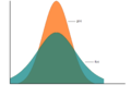
At the tails, f(x)/g(x) may become very large.
-
f(x) and g(x) should have similar shapes. This scenario could be problematic with importance sampling.


A bad choice for g(x) can cause a problem and a good choice can reduce the variance. Therefore we need to have criteria for choosing good [math]\displaystyle{ g }[/math]:
Advice 1: Choose [math]\displaystyle{ g }[/math] such that [math]\displaystyle{ g }[/math] has thicker tails compared to [math]\displaystyle{ f }[/math]
- Also, if over a set [math]\displaystyle{ A }[/math], [math]\displaystyle{ g }[/math] is small but [math]\displaystyle{ f }[/math] is large, then [math]\displaystyle{ \frac {f(x)}{g(x)} }[/math] could be large. (i.e. the variance could be large.)
Advice 2: Choose [math]\displaystyle{ g }[/math] to have similar shape with [math]\displaystyle{ f }[/math]
-In general, it is better to choose [math]\displaystyle{ g }[/math] such that it is similar to [math]\displaystyle{ f }[/math] in terms of shape but with thicker tails.
Example List
Estimate [math]\displaystyle{ \displaystyle I = Pr(Z\gt 3),\ \text{ where }\ Z \sim N(0,1) }[/math]
Note:[math]\displaystyle{ \displaystyle Pr(Z\gt 3)=Pr(Z\lt -3) }[/math] due to the symmetric property of normal distribution. The occurrence of Z>3 is a rare event since [math]\displaystyle{ \displaystyle Pr(Z\gt 3) }[/math] is roughly 0.13% (this is obtained from a normal probability table). stat 231 note.
Method 1: Basic Sampling
We let [math]\displaystyle{ \displaystyle f(x) }[/math] be the pdf of the standard normal. We want to compute
[math]\displaystyle{ I=\int^{\infty}_3 f(x)\,dx =\int_{- \infty}^{\infty} h\left( x\right) f\left( x\right) dx }[/math]
where
[math]\displaystyle{
h(x) = \begin{cases}
1, & \text{if } x \gt 3 \\
0, & \text{if } x \leq 3
\end{cases} }[/math]
[math]\displaystyle{ \ ,\ f(x) = \frac{1}{\sqrt{2\pi}}e^{-\frac{1}{2}x^2} }[/math]
This gives [math]\displaystyle{ \widehat{I} = \frac{1}{n} \sum_{i = 1}^{n} h({x_{i})} }[/math] where [math]\displaystyle{ x_{i} ~\sim N(0,1) }[/math]
which is equivalent to [math]\displaystyle{ \widehat{I}= \frac{\text{number of observations }\gt 3}{n} }[/math]
Note :we could also formulate [math]\displaystyle{ h(x) }[/math] to be the following because the density at a single point (3 in this case) is 0 anyways.
[math]\displaystyle{
h(x) = \begin{cases}
1, & \text{if } x \geq 3 \\
0, & \text{if } x \lt 3
\end{cases} }[/math]
MATLAB Code
x=randn(1,100);
sum(x>3)/100;

clc
clear all
close all
n = 100;
for ii = 1:200;
     x = randn(1,n);
     I(ii) = sum(x>3)/n %%sums values in x vector greater than 3 and divides by n
end
Note: (x>3) is an indicator function in Matlab.
It will provide answers in the form of boolean.
In this example,
We see that if we repeat I(ii) several times, we get 0, 0, 0.01, 0, 0, 0.
This is considered a very good result as 5 out of 6 times you get the actual mean of the distribution.
Method 2: Importance Sampling
[math]\displaystyle{ I=\int h\left( x\right) f\left( x\right) dx= \int \frac{h(x)f(x)}{g(x)} g(x) dx }[/math]
where [math]\displaystyle{ \frac{h(x)f(x)}{g(x)} = w(x) }[/math] Choose [math]\displaystyle{ g(x) }[/math] from [math]\displaystyle{ N(4,1) }[/math]
Note :
- [math]\displaystyle{ N(4,1) }[/math] was chosen according to our advice mentioned earlier. [math]\displaystyle{ N(4,1) }[/math] has the same shape (actually the exact same shape) as [math]\displaystyle{ N(0,1) }[/math]. Hence it will not increase the variance of our simulation.
- The reason why we do not choose uniform distribution for this case is because the uniform distribution only distributed over a finite interval from a to b, where the required [math]\displaystyle{ N(4,1) }[/math] distributed over all x.
- To be more precise, we can see that choosing a distribution centered at 3 or nearby points (i.e. 2 or 4) will help us generate more points which are greater than 3. Thus the size of variance between different samples will be reduced. The reason behind this can be explained as follows:
Eg: If we take a sample of 1000 points and very few points are above three and we take the sample again, we will have a huge variance as the probability of samples greater than 3 is low. We may even get 0 as our simulated answer as shown in class which is not the case. Thus using this method helps us overcome the problem of sampling from rare events.
[math]\displaystyle{ \widehat{I} = \frac{1}{n} \sum_{i = 1}^{n} w({x_{i})} }[/math] where [math]\displaystyle{ x_{i} ~\sim N(4,1) }[/math]
[math]\displaystyle{ \frac{f(x)}{g(x)}=\dfrac {e^{-\dfrac{x^{2}} {2} }} {e^{-\dfrac{{(x-4)}^{2}}{2} }} =e^{8-4x} }[/math]
This gives [math]\displaystyle{ \displaystyle w(x)=h(x) e^{8-4x} }[/math]
MATLAB
clear all
close all
clc  %% clc clears all input and output from the Command Window display, giving you a "clean screen."
n=100;
for ii=1:200
   x=randn(1,n);
   lb(ii)=sum(x>3)/n; %sums values in x vector greater than 3 and divides by n

   x=randn(1,n)+4;
   ls(ii)=sum((x>3).*exp(8-4*x))/n; %w(x)/n
end
var(lb)
var(ls)
var(ls)/var(lb)
hist(ls,50)
.jpg)
Note:
The helper g(x) needs to be a valid pdf.
Example3
If [math]\displaystyle{ g(x)=x }[/math] for x belongs to [math]\displaystyle{ [0,1] }[/math], the integral of this function is not 1.
So, we need to add a constant number to make it a valid pdf.
Therefore, we change it to [math]\displaystyle{ g(x)=2x }[/math] for 0<x<1
This code is for calculating the variance.
The first method produced a variance with a power of 10-5, while the second method produced a variance with a power of 10-8. Hence, a clear variance reduction is evident.
Side Note:
- The most effective variance reduction technique is to increase the sample size. For instance, in the above example, by using Importance Sampling, we are able to reduce the variance by 3 degrees of power.
- However if we used Method 1 while increasing the sample size from 200 to 1,000,000 or more, we are able to decrease the variance by 4 or more degrees of power.
- Also, note that since there is a large variance, it is problematic. So by choosing a different distribution that is not centered around 0, a distribution that is centered at 4 for example would result in less variation. For example, choose [math]\displaystyle{ \displaystyle g(x)\sim N(4,1) }[/math]
Important Notes on selection of g(x):
- g(x) must have the same support as f(x) in order for accurate sampling
- g(x) must be such that it encourages the occurrence of rare points (rare h(x))
- Selection of g(x) greatly affects E[w2] therefore affects the variance. A poor choice of g(x) can cause a significant increase in the variance, thus defeating the purpose of Importance Sampling.
- Specifically, it is recommended that g(x) have the following properties<ref>
http://ib.berkeley.edu/labs/slatkin/eriq/classes/guest_lect/mc_lecture_notes.pdf </ref>
1) It is greater than 0 whenever the function in question is not zero.
2) It should be close to being proportional to the absolute value of the function in question.
3) It should be easy to simulate.
4) It should be easy to compute for any realizable x.
- Although there are many methods of variance reduction, the best way is to increase n. The larger n is, the closer your value is to the exact value.
- Using various computer software is the most effective method of reducing a variance.
Class 24, Thursday, July 25, 2013
Importance Sampling
Importance Sampling is the most fundamental variance reduction technique, and often leads to a dramatic variance reduction.
Importance sampling involves choosing a sampling distribution that favor important samples*.(Simulation and the Monte Carlo Method, Reuven Y. Rubinstein)
- Here "favor important samples" means to encourage the occurrence of the desired event or part of the desired event. For instance, if the event of interest is rare (probability of occurrence is close to zero), we "favor important samples" by choosing a sampling distribution such that the event has higher probability of occurrence.
Definition of importance sampling from Wikipedia:
Importance sampling is a general technique for estimating properties of a particular distribution, while samples are generated from a different distribution other than the distribution of interest. It is related to umbrella sampling in computational physics. Depending on the application, the term may refer to the process of sampling from this alternative distribution, the process of inference, or both.
Recall that using importance sampling,we have the following:
[math]\displaystyle{ I=\int_{a}^{b}f(x)dx = \int_{a}^{b}f(x)(b-a) \times \frac{1}{b-a}dx }[/math]
If g(x) is another probability density function,
note: in summary, a good importance sampling function g(x) should satisfies:
1. g(x) > 0 whenver f(x)not equal to 0
2. g(x) should be equal or close to the absolute value of f(x)
3. easy to simulate values from g(x)
4. easy to compute the density of g(x)
original source is here
http://ib.berkeley.edu/labs/slatkin/eriq/classes/guest_lect/mc_lecture_notes.pdf
then we have:
[math]\displaystyle{ I = \int h(x)f(x)\,dx =\int\frac{h(x)f(x)}{g(x)}\times g(x)\,dx }[/math], where [math]\displaystyle{ w(x) = \frac{h(x)f(x)}{g(x)} }[/math]
In order to estimate I we have:
[math]\displaystyle{ \widehat{I}=\frac{1}{n}\sum_{i=1}^{n}w(x) }[/math] and [math]\displaystyle{ g^{*}(x) = \frac{|h(x)|f(x)}{\int |h(x)|f(x)dx} }[/math], where [math]\displaystyle{ h(x)\gt =0 }[/math] for all x
Higher values of n correspond to values of [math]\displaystyle{ \widehat{I} }[/math] closer to [math]\displaystyle{ {I} }[/math], which approaches [math]\displaystyle{ \widehat{I} }[/math] as n approaches infinity.
Note: g(x) should be chosen carefully. It should be easy to sample from. Also, since this method is for minimizing the variance, g(x) should be chosen in a manner such that the variance is minimized. g*(x) is the distribution that minimizes the variance.
- In assignment 6, we need to prove that "the choice of g that minimizes the variance of I is g*(x)". Furthermore, we were asked to minimize the variance of I which requires us to minimize the variance of w (as seen below). For simplicity, we assume that h(x) is greater than or equal to 0 for all x. In reality, h(x) can be positive, negative or 0.
- [math]\displaystyle{ \, Var(x) = E(x^2) - (E(x))^2 }[/math]
- [math]\displaystyle{ \, Var(I) = Var(\frac{1}{n} \sum_{i = 1}^{n} w({x_{i})})= Var(w)/n }[/math]
Note: This expression has equivalent to the summation of all variances of W, because W’s are independent, hence covariance terms are zero.
- [math]\displaystyle{ \, Var(w) = E(w^2) - (E(w))^2 }[/math]
- [math]\displaystyle{ = \int(\frac{h(x)f(x)}{g(x)})^2 g(x) dx - (\int\frac{h(x)f(x)}{g(x)} g(x) dx)^2 }[/math]
- The Second Term
- [math]\displaystyle{ \left(\int \frac{h(x)f(x)}{g(x)}g(x)dx\right)^2=\left(\underbrace{\int h(x)f(x)dx}_I\right)^2=I^2 }[/math]
- Note : No matter what g is, the second term is always constant with respect to g at [math]\displaystyle{ I^2 }[/math].
since [math]\displaystyle{ I^2 }[/math] is constant with respect to g, if we want to minimize the variance, we only need to consider the first term.
So, we need to minimize the first term.
- The First Term
[math]\displaystyle{ \int(\frac{h(x)f(x)}{g(x)})^2 g(x) dx }[/math]
[math]\displaystyle{ = \int\frac{h(x)^2f(x)^2}{g(x)} dx }[/math]
If [math]\displaystyle{ h(x) \geq 0 }[/math], then [math]\displaystyle{ g^*(x)= \frac{h(x)f(x)}{\int h(x)f(x) dx} = \frac{h(x)f(x)}{I} }[/math] where [math]\displaystyle{ I = \int h(x)f(x) dx }[/math]
[math]\displaystyle{ = \int\frac{h(x)^2f(x)^2}{\frac{h(x)f(x)}{I}} dx }[/math]
[math]\displaystyle{ = \int\frac{I \times h(x)^2f(x)^2}{h(x)f(x)} dx }[/math]
[math]\displaystyle{ = \int I \times h(x)f(x) dx }[/math]
[math]\displaystyle{ = I\times \left(\underbrace{\int h(x)f(x)dx}_I\right) }[/math]
[math]\displaystyle{ = I^2 }[/math]
(because we choose g(x)=g*(x))
[math]\displaystyle{ I = \int h(x)f(x) dx \leq \int |h(x)|f(x) dx }[/math]
since [math]\displaystyle{ f(x) \geq 0 }[/math], [math]\displaystyle{ |h(x)| \geq h(x) }[/math]
Therefore, at [math]\displaystyle{ \,g(x), Var(w)=I^2 -I^2=0 }[/math]
Note that although this proof uses the assumption of h(x) ≥ 0, the result still holds for functions h(x) that are not always non-negative (however, the variance will not be 0)
More specifically, since [math]\displaystyle{ \int |h(x)|f(x) dx \geq \int h(x)f(x) dx = I }[/math] where [math]\displaystyle{ h(x) }[/math] can be negative, so [math]\displaystyle{ \, Var(w) \geq I^2-I^2 = 0 }[/math], and as a result Var(w) will always be non-negative.
Remark: Since [math]\displaystyle{ I^2 }[/math] is constant of g, we only consider minimizing the first term to minimize the variance.
Normalized Importance Sampling
[math]\displaystyle{ I= \frac{\int h(x)f(x) dx}{\int f(x) dx} }[/math] since f(x) is a pdf, and the integral is just equal to 1
[math]\displaystyle{ =\frac{\int\frac{ h(x)f(x)}{g(x)}g(x)dx}{\int \frac{f(x)g(x)}{g(x)}dx} }[/math]
[math]\displaystyle{ \hat{I}= \frac{1}{n}\sum_{i=1}^{n}\frac{h(x_i)f(x_i)}{g(x_i)} =\frac{1}{n}\sum_{i=1}^{n}h(x_i)\beta_i^* }[/math] where [math]\displaystyle{ \beta_i^* = \frac{\beta_i}{\sum_{i=i}^{n}\beta_i} }[/math] and [math]\displaystyle{ \beta_i = \frac{f(x_i)}{g(x_i)} }[/math]
Where [math]\displaystyle{ \frac{f(x)}{g(x)} }[/math] corresponds to a weight.
[math]\displaystyle{ \,\beta = [\beta_1,\beta_2, ......, \beta_n] }[/math] xi~[math]\displaystyle{ g(x) }[/math]
[math]\displaystyle{ \beta_i^*= \biggl[ \frac{\beta_1}{\beta_1+...+\beta_n}, \frac{\beta_2}{\beta_1+...+\beta_n}, ... , \frac{\beta_n}{\beta_1+...+\beta_n} \biggr] }[/math]
Note: Above is not included in exam.
- Note:
- One advantage of using Normalized Importance Sampling is that we don't need to know the normalization factor of distribution f(x). The normalization will be applied to the individual [math]\displaystyle{ \beta_i }[/math], and so the sum of the [math]\displaystyle{ \beta }[/math]'s will be of the same proportion.
- The normalization factor will be cancelled out when we calculate the weights. Note that this is the same advantage as that of Metropolis Hastings. It is a powerful advantage because in practice, determining the normalizing constant can be very difficult. This advantage does not hold when using [math]\displaystyle{ \beta }[/math] only [math]\displaystyle{ \beta^* }[/math]
- Normalized Importance Sampling however, performs worse than regular importance sampling as we are approximating the normalizing constant
- One advantage of using Normalized Importance Sampling is that we don't need to know the normalization factor of distribution f(x). The normalization will be applied to the individual [math]\displaystyle{ \beta_i }[/math], and so the sum of the [math]\displaystyle{ \beta }[/math]'s will be of the same proportion.
Here is a video explaining normalized importance sampling sightly differently.
Final Exam Review
Summary of Final Exam Topics: Pre-Midterm: • Multiplicative Congruential Algorithm • Inverse Transform Method • Acceptance Rejection Method • Multivariate Random Variable Generation • Vector Acceptance Rejection Method Post-Midterm: • Poisson Process • Markov Chains (MC) • Page Rank (MC Application) • Markov Chain Monte Carlo (MCMC) • Metropolis-Hasting Algorithm (MCMC Application) • Simulated Annealing (MCMC Application) • Gibbs Sampling (Metropolis-Hasting adaptation) • Monte Carlo Integration • Importance Sampling
Only review of material not covered on the midterm, the final will be cumulative
For review of material covered on the midterm refer to class 12 - June 13th.
Stochastic Processes (we learned Poisson Process and Markov Chain).
- {Xt | t in T}
where xt is an element of state space X and T is the index set.
- A collection of random variables.
- The two most important stochastic processes we looked at in this term are Poission Process and Markov Chain.
===Poisson Process=== (useful for counting number of arrivals):
- two assumptions:
- the number of arrivals in non-overlapping intervals are independent
- the number of arrivals in an interval I is Poisson distributed.
- the mean of the Poisson Process is [math]\displaystyle{ \lambda \times length(I) }[/math]
- Can be generated using the exponential distribution
Algorithm<br\>
- 1. Set n=1, a=1<br\>
- 2. [math]\displaystyle{ U_n }[/math] ~ [math]\displaystyle{ U[0,1] }[/math] and set [math]\displaystyle{ a=aU_n }[/math]<br\>
- 3. If [math]\displaystyle{ a \geq e^{-\lambda} }[/math] then: n=n+1 and go to Step 2. Else set X=n-1.
Acknowledgments: from Spring 2012 stat 340 coursenotes
Matlab code review:
T(1)=0;
ii=1;
l=2;
TT=5;
while T(ii)<=TT
   u=rand;
   ii=ii+1;
   T(ii)=T(ii-1) - (1/l)*log(u);
end
plot(T, '.')
Markov Chain:
Recall that:
- A Markov Chain is a discrete random process which transits from one state to another. The number of states in a Markov Chain can be finite or countable.
- A Markov Chain has the Memoriless Property:
[math]\displaystyle{ Pr(X_t=x_t|X_{t-1}=x_{t-1},..., X_1=x_1)= Pr(X_t=x_t|X_{t-1}=x_{t-1}) }[/math].
In other words, the current state only depends on the previous state and no other prior states. This property is also called the "Markov property".
- The possible values of Xi are called the "state space" of the chain.
- Transition probability Pij = Pr {xt+1=j | xt = i} = P(i,j)
- Transition matrix P = [P11 ... P1n ; ... ; Pn1 ... Pnn]. where P ij >= 0, row sum = 1
- N-step transition matrix Pn(i,j) = Pr {xt+n=j | xt = i}, Pn = Pn
- Marginal distribution:[math]\displaystyle{ \mu_1~ = \mu_0P }[/math]
In general, [math]\displaystyle{ \mu_n~ = \mu_0P^n }[/math]
- Stationary distribution: [math]\displaystyle{ \pi }[/math] = [math]\displaystyle{ \pi }[/math] P
- Limiting distribution:
[math]\displaystyle{ \lim_{n\to \infty} P^n= \left[ {\begin{array}{ccc}
\pi_1 \\
\vdots \\
\pi_n \\
\end{array} } \right] }[/math]
- Detailed Balance:
Detailed Balance
if [math]\displaystyle{ \pi }[/math]i Pij = [math]\displaystyle{ \pi }[/math]j Pji,
[math]\displaystyle{ [\pi P][\pi P]j = \sum \pi }[/math] i Pij [math]\displaystyle{ = \sum \pi }[/math]jPji [math]\displaystyle{ = \pi }[/math]j[math]\displaystyle{ \sum P }[/math]ji [math]\displaystyle{ = \pi }[/math]j
Proof: We will look at a single row from
[math]\displaystyle{ \; \pi P }[/math], denoted by [math]\displaystyle{ \; [\pi P]_j }[/math]
[math]\displaystyle{ \; [\pi P]_j = \sum_i \pi_i P_{ij} =\sum_i P_{ji}\pi_j =\pi_j\sum_i P_{ji} =\pi_j ,\forall j }[/math]
note: [math]\displaystyle{ \sum_i P_{ji}=1. }[/math]
- Application of Markov Chain - PageRank:
[math]\displaystyle{ P_i= (1-d) + d\cdot \sum_j \frac {L_{ij}P_j}{c_j} }[/math], where 0 < d < 1 is constant
where [math]\displaystyle{ L_{ij} }[/math] is 1 if j has link to i, and 0 otherwise;
[math]\displaystyle{ C_j = \sum_i L_{ij} }[/math]
Note: we solved this using systems of equations or eigenvalues and eigenvectors
Matrix form:
[math]\displaystyle{ P=[(1-d)~\frac{ee^T}{N}+dLD^{-1}]P }[/math]
(ee^T is a matrix of all 1s)
[math]\displaystyle{ P=AP , where A=[(1-d)~\frac{ee^T}{N}+dLD^{-1}] }[/math]
The matrix has column summation equals to one and has eigenvalues equal to one.
Markov Chain Monte Carlo (MCMC):
-Recall that MCMC is a special form of stochastic process where Xt depends only on Xt-1
-The two applications of MCMC are Metropolis–Hasting algorithm and Simulated Annealing.
- 'Metropolis–Hasting Algorithm':
If we have target distribution f, which we want to sample from, then
decide to accept the sample or reject.
1) X0= state of chain at time 0. Set i = 0
2) [math]\displaystyle{ Y }[/math]~[math]\displaystyle{ q(y|x) }[/math]
3) [math]\displaystyle{ r(x,y)=\min\{\frac{f(y)}{f(x)}\frac{q(x|y)}{q(y|x)},1\} }[/math]
4) [math]\displaystyle{ U }[/math]~[math]\displaystyle{ U(0,1) }[/math]
5) If [math]\displaystyle{ U\lt r }[/math], [math]\displaystyle{ X_{t+1}=Y }[/math]; else [math]\displaystyle{ X_{t+1}=X_t }[/math]
6) i = i + 1. Return to Step 2.
Note :for just the Metropolis Algorithm everything is the same as in Metropolis-Hasting Algorithm except that step 3 is:
[math]\displaystyle{ r(x,y)=\min\{\frac{f(y)}{f(x)},1\} }[/math] This is because q is symmetric in the Metropolis Algorithm.
- Application of M.H. Algorithm - Simulated Annealing:
min h(x) = max exp(-h(x)/T)
Simulated Annealing Algorithm:
1) Set T to be a large number, Set i = 0, [math]\displaystyle{ X_{t} }[/math] = 0
2) [math]\displaystyle{ Y }[/math]~[math]\displaystyle{ Q(Y|X) }[/math]
3) [math]\displaystyle{ r(x,y) = \min\{\frac{f(y)}{f(x)},1\} }[/math]
Since q(.) is symetric
4) [math]\displaystyle{ U }[/math]~[math]\displaystyle{ U(0,1) }[/math]
5) If [math]\displaystyle{ U\lt r }[/math], [math]\displaystyle{ X_{t+1}=Y }[/math]; else [math]\displaystyle{ X_{t+1}=X_t }[/math]
6) Decrease T. Return to Step 2.
- note: popular candidates for Q(Y|X) are uniform distribution and normal distribution.(symmetric)
- Proof of MH Algorithm (convergence):
Detailed Balance: [math]\displaystyle{ f(x) P(y|x) = f(y) P(x|y) }[/math]
1) [math]\displaystyle{ \frac {f(y) q(x|y)}{f(x) q(y|x)}\lt 1 }[/math]
=> r(x,y) = [math]\displaystyle{ \frac {f(y)q(x|y)}{f(x)q(y|x)} }[/math]
2) [math]\displaystyle{ \frac {f(y)q(x|y)}{f(x)q(y|x)}\gt 1 }[/math]
=> r(x,y) = 1
LHS: [math]\displaystyle{ f(x)P(y|x)= f(x)q(y|x)r(x,y) }[/math]
=f(x)q(y|x)[math]\displaystyle{ \frac {f(y)q(x|y)}{f(x)q(y|x)} }[/math]
=f(y)q(x|y)
[math]\displaystyle{ \begin{align}
\text{RHS} & = f(x)P(x|y)= f(x)q(x|y)r(y,x) \\
& =f(x)q(x|y)*1 \\
& =f(y)q(x|y) = \text{LHS}
\end{align} }[/math]
- Therefore, detailed balance is satisfied, so f(x) is a stationary distribution!
- We can also prove similarly for Metropolis Hasting and Simulated Annealing (even easier since they don't have q(x|y)/q(y|x) when calculating r)
- Proof of Simulated Annealing Algorithm (convergence):
Detailed Balance: [math]\displaystyle{ \,f(x) P(y|x) = f(y) P(x|y) }[/math]
Since q(y|x) is symmetric -> q(y|x)=q(x|y)
1) [math]\displaystyle{ \frac {f(y)}{f(x)}\lt 1 }[/math]
=> [math]\displaystyle{ r(x,y) = \frac {f(y)}{f(x)} }[/math]
2) [math]\displaystyle{ \frac {f(y)}{f(x)}\gt 1 }[/math]
=> [math]\displaystyle{ \, r(x,y) = 1 }[/math]
[math]\displaystyle{ \begin{align}
\text{LHS} & = f(x)P(y|x)= f(x)q(y|x)r(x,y) \\
& =f(x)q(y|x)\frac {f(y)}{f(x)} \\
& =f(y)q(x|y) \end{align} }[/math]
[math]\displaystyle{ \begin{align}
\text{RHS} & = f(y)P(x|y)= f(y)q(x|y)r(y,x) \\
& =f(y)q(x|y)\times 1 \\
& =f(y)q(x|y) = \text{LHS}
\end{align} }[/math]
Gibbs Sampling:
The most widely used version of the Metropolis-Hastings algorithm is the Gibbs sampler.
This sampling method is useful when dealing with multivariable distributions.
[math]\displaystyle{ f(x_1, x_2, ..., x_d) }[/math]
[math]\displaystyle{ x = (x_1, ..., x_d) }[/math]
- Suppose [math]\displaystyle{ x_t = (x_{t_1}, ..., x_{t_d}) }[/math] are the initial values.
Start by sampling from [math]\displaystyle{ x_1 }[/math]:
[math]\displaystyle{ \displaystyle Y_1 \sim f(x_1 | x_{t_2}, ..., x_{t_d}) }[/math]
[math]\displaystyle{ \displaystyle Y_i \sim f(x_i | Y_1, ..., Y_{i-1}, x_{t_{i+1}}, ..., x_{t_d}) }[/math], where [math]\displaystyle{ i=2, ..., d }[/math]
[math]\displaystyle{ \displaystyle Y_d \sim f(x_d | Y_1, ..., Y_{d-1}) }[/math]
Example:
Consider a biased die [math]\displaystyle{ \pi }[/math]= [0.1, 0.1, 0.3, 0.3, 0.1, 0.1]
We use [math]\displaystyle{ 6 x 6 }[/math] matrix [math]\displaystyle{ \mathbf{Q} }[/math] as the proposal distribution
And we use U(0,1) distribution.
[math]\displaystyle{ \mathbf{Q} =
\begin{bmatrix}
1/6 & 1/6 & \cdots & 1/6 \\
1/6 & 1/6 & \cdots & 1/6 \\
\vdots & \vdots & \ddots & \vdots \\
1/6 & 1/6 & \cdots & 1/6
\end{bmatrix}
}[/math]
Algorithm
1. [math]\displaystyle{ x_t=5 }[/math]
2. Y~unif[1,2,...,6]
3. [math]\displaystyle{ r_{ij} = \min \{\frac{\pi_j q_{ji}}{\pi_i q_{ij}}, 1\} = \min \{\frac{\pi_j 1/6}{\pi_i 1/6}, 1\} = \min \{\frac{\pi_j}{\pi_i}, 1\} }[/math]
4. U~Unif(0,1)
if [math]\displaystyle{ u \leq r_{ij} }[/math], Xt+1=Y
else Xt+1=Xt
go back to 2
Monte Carlo Integration
- It is a technique used for numerical integration using random numbers.
- This method is one of the Monte Carlo methods that numerically computes definite integrals.
- The above integral can be rewritten as following:
[math]\displaystyle{ I = \int_a^b h(x)dx = \int_a^b h(x) \frac{b-a}{b-a} dx = \int_a^b \frac{h(x)}{b-a} (b-a) dx }[/math] where [math]\displaystyle{ U(a,b) = 1/(b-a) }[/math]
So we have [math]\displaystyle{ w(x)= \frac{h(x)}{b-a} }[/math] and [math]\displaystyle{ \hat{I} = \frac{1}{n} \sum_{i=1}^n w(x_i),x_i \sim U(a,b) }[/math]
For the case where we do not have finite bounds on the integration, we have
[math]\displaystyle{ I = \int h(x)f(x)dx }[/math]
[math]\displaystyle{ \hat{I} = \frac{1}{n} \sum _{i=1}^n h(x_i) , \text{where} \ x_i \sim f }[/math]
Importance Sampling
Importance Sampling is a useful technique for variance reduction.
Using importance sampling, we have:
[math]\displaystyle{ I=\int_{a}^{b}f(x)dx = \int_{a}^{b}f(x)(b-a) \times \frac{1}{b-a}dx }[/math]
If g(x) is another probability density function,
[math]\displaystyle{ I = \int h(x)f(x)\,dx =\int\frac{h(x)f(x)}{g(x)}\times g(x)\,dx }[/math], where [math]\displaystyle{ w(x) = \frac{h(x)f(x)}{g(x)} }[/math]
To approximate I,
[math]\displaystyle{ \widehat{I}=\frac{1}{n}\sum_{i=1}^{n}w(x) }[/math] and [math]\displaystyle{ g^{*}(x) = \frac{|h(x)|f(x)}{\int |h(x)|f(x)dx} }[/math], where [math]\displaystyle{ h(x)\gt =0 }[/math] for all x
Note: g(x) should be chosen carefully so that its distribution would minimize the variance.