From Variational to Deterministic Autoencoders
Presented by
John Landon Edwards
Introduction
This paper presents an alternative framework to the stochastic Variational Autoencoders (VAEs) that is deterministic named the Regularized Autoencoders (RAEs) for generative modeling. The goal of VAEs is to learn from a large collection of high-dimensional samples to draw new sample from the inferred population distribution. RAEs hope to achieve the same goal without the drawbacks of VAEs in practice. The advantages of RAEs to VAEs are that they are easier to train and simpler. The paper investigates how forcing an arbitrary prior [math]\displaystyle{ p(z) }[/math] within VAEs could be substituted instead with a regularization scheme to the loss function. Furthermore, a generative mechanism for RAEs is proposed utilizing an ex-post density estimation step that can also be applied to existing VAEs. Finally, they conduct an empirical comparison between VAEs and RAEs to demonstrate that the latter are able to generate samples that are comparable or better when applied to domains of images and structured objects.
Motivation
The authors point to several drawbacks currently associated with VAE's including:
- the compromise between sample quality and reconstruction quality is poor
- over-regularisation induced by the KL divergence term within the objective [5]
- posterior collapse in conjunction with powerful decoders [1]
- increased variance of gradients caused by approximating expectations through sampling [3][7]
- learned posterior distribution doesn't match the latent assumption [8]
These issues motivate their consideration of alternatives to the variational framework adopted by VAE's.
Furthermore, the authors note that VAE's introduction of random noise within the reparameterization [math]\displaystyle{ z = \mu(x) +\sigma(x)\epsilon }[/math] have a regularization effect because it promotes the learning of a smoother latent space. This motivates their exploration of regularization schemes within an autoencoders loss function which could substitute the VAE's random noise injection. This would allow for the elimination of the variational framework and to circumvent its associated drawbacks.
Due to the deterministic nature of RAES, it is impossible to sample from [math]\displaystyle{ p(z) }[/math] to produce generated samples. The authors provide a solution to this problem by fitting a density estimate of the latent post-training to generate new samples.
Related Work
The authors point to similarities between their framework and Wasserstein Autoencoders (WAEs) [5] where a deterministic version can be trained. However, the RAEs utilize a different loss function and differs in their implementation of the ex-post density estimation. Additionally, they suggest that Vector Quantized-Variational AutoEncoders (VQ-VAEs) [1] can be viewed as deterministic. VQ-VAES also adopt ex-post density estimation but implement this through a discrete auto-regressive method. Furthermore, VQ-VAEs utilize a different training loss that is non-differentiable.
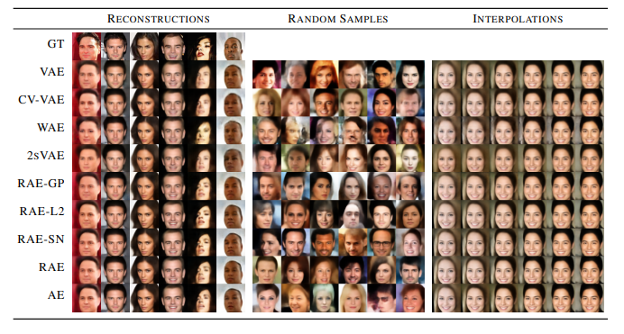
The following figure summarizes the qualitative performance of the various methods in related work. Looking at sample quality for VAEs, WAEs, 2sVAEs, RAEs and CelebA; RAEs can be seen to have a slight edge in terms of sharpness of samples and their reconstructions with smooth interpolation into the latent space.

Framework Architecture
Overview
The Regularized Autoencoder proposes three modifications to the existing VAEs framework. Firstly, eliminating the injection of random noise [math]\displaystyle{ \epsilon }[/math] from the reparameterization of the latent variable [math]\displaystyle{ z }[/math]. Secondly, it proposes a resigned loss function [math]\displaystyle{ \mathcal{L}_{RAE} }[/math]. Finally, it proposes an ex-post density estimation procedure for generating samples from the RAE.
Eliminating Random Noise
The authors proposes eliminating the injection of random noise [math]\displaystyle{ \epsilon }[/math] from the reparameterization of the latent variable [math]\displaystyle{ z = \mu(x) +\sigma(x)\epsilon }[/math] resulting in a Encoder [math]\displaystyle{ E_{\phi} }[/math] that deterministically maps a data point [math]\displaystyle{ x }[/math] to a latent variable [math]\displaystyle{ z }[/math].
The current variational framework of VAEs enforces regularization on the encoder posterior through KL-divergence term of its training loss function: \begin{align} \mathcal{L}_{ELBO} = \mathbb{E}_{z \sim q_{\phi}(z|x)}\log p_{\theta}(x|z) + \mathbb{KL}(q_{\phi}(z|x) | p(z)) \end{align}
In eliminating the random noise within [math]\displaystyle{ z }[/math] the authors suggest substituting the losses KL-divergence term with a form of explicit regularization. This makes sense because [math]\displaystyle{ z }[/math] is no longer a distribution and [math]\displaystyle{ p(x|z) }[/math] would be zero almost everywhere. Also as the KL-divergence term previously enforced regularization on the encoder posterior so its plausible that an alternative regularization scheme could impact the quality of sample results. This substitution of the KL-divergence term leads to redesigning the training loss function used by RAEs.
Redesigned Training Loss Function
The resigned loss function [math]\displaystyle{ \mathcal{L}_{RAE} }[/math] is defined as: \begin{align} \mathcal{L}_{RAE} = \mathcal{L}_{REC} + \beta \mathcal{L}^{RAE}_Z + \lambda \mathcal{L}_{REG}\\ \end{align} where [math]\displaystyle{ \lambda }[/math] and [math]\displaystyle{ \beta }[/math] are hyper parameters.
The first term [math]\displaystyle{ \mathcal{L}_{REC} }[/math] is the reconstruction loss, defined as the mean squared error between input samples and their mean reconstructions [math]\displaystyle{ \mu_{\theta} }[/math] by a decoder that is deterministic. In the paper it is formally defined as: \begin{align} \mathcal{L}_{REC} = ||\mathbf{x} - \mathbf{\mu_{\theta}}(E_{\phi}(\mathbf{x}))||_2^2 \end{align} However, as the decoder [math]\displaystyle{ D_{\theta} }[/math] is deterministic the reconstruction loss is equivalent to: \begin{align} \mathcal{L}_{REC} = ||\mathbf{x} - D_{\theta}(E_{\phi}(\mathbf{x}))||_2^2 \end{align}
The second term [math]\displaystyle{ \mathcal{L}^{RAE}_Z }[/math] is defined as : \begin{align} \mathcal{L}^{RAE}_Z = \frac{1}{2}||\mathbf{z}||_2^2 \end{align} This is equivalent to constraining the size of the learned latent space, which prevents unbounded optimization.
The third term [math]\displaystyle{ \mathcal{L}_{REG} }[/math] acts as the explicit regularizer to the decoder. The authors consider the following potential formulations for [math]\displaystyle{ \mathcal{L}_{REG} }[/math]
- Tikhonov regularization(Tikhonov & Arsenin, 1977)
\begin{align} \mathcal{L}_{REG} = ||\theta||_2^2 \end{align}
- Gradient Penalty:
\begin{align} \mathcal{L}_{REG} = ||\nabla_{x} D_{\theta}(E_\phi(x)) ||_2^2 \end{align}
- Spectral Normalization:
- The authors also consider using Spectral Normalization in place of [math]\displaystyle{ \mathcal{L}_{REG} }[/math] whereby each weight matrix [math]\displaystyle{ \theta_{\ell} }[/math] in the decoder network is normalized by an estimate of it largest singular value [math]\displaystyle{ s(\theta_{\ell}) }[/math]. Formally this is defined as:
\begin{align} \theta_{\ell}^{SN} = \theta_{\ell} / s(\theta_{\ell})\\ \end{align}
Ex-Post Density Estimation
Recall that since the autoencoder is no longer stochastic, it may prove to be a challenge to sample from the latent space to generate new samples. However, the author proposes to fit a density estimator [math]\displaystyle{ q_{\delta}(\mathbf{z}) }[/math] over the trained latent spaces points [math]\displaystyle{ \{\mathbf{z}=E_{\phi}(\mathbf{x})|\mathbf{x} \in \chi\} }[/math] to solve this problem. They can then sample using the estimated density to produce decoded samples. The authors note the choice of density estimator here needs to balance a trade-off of expressiveness and simplicity whereby a good fit of the latent points is produced but still allowing for generalization to untrained points. It is noteworthy that, even in VAE where one would sample from the prespecified [math]\displaystyle{ p(z) }[/math], the generative mechanism is not perfect either, as often times the posterior [math]\displaystyle{ q_{\phi}(z) }[/math] can depart a lot from [math]\displaystyle{ p(z) }[/math] and thus the sampled [math]\displaystyle{ z }[/math] might fall into regions that the decoder hasn't seen. Therefore, intuitively the use of an estimated density is not likely to be more compromising than [math]\displaystyle{ p(z) }[/math] already is in VAE.
Empirical Evaluations
Image Modeling:
Models Evaluated:
The authors evaluate regularization schemes using Tikonov Regularization , Gradient Penalty, and Spectral Normalization. These correspond with models (RAE-L2) ,(RAE-GP) and (RAE-SN) respectively, as seen in figure 1. Additionally they consider a model (RAE) where [math]\displaystyle{ \mathcal{L}_{REC} }[/math] is excluded from the loss and a model (AE) where both [math]\displaystyle{ \mathcal{L}_{REC} }[/math] and [math]\displaystyle{ \mathcal{L}^{RAE}_{Z} }[/math] are excluded from the loss. For a baseline comparison they evaluate a regular Gaussian VAE (VAE), a constant-variance Gaussian (CV-VAE) VAE, a Wassertien Auto-Encoder (WAE) with MMD loss, and a 2-stage VAE [2] (2sVAE).
Metrics of Evaluation:
Each model was evaluated on the following metrics:
- Rec: Test sample reconstruction where the French Inception Distance (FID) is computed between a held-out test sample and the networks outputted reconstruction.
- [math]\displaystyle{ \mathcal{N} }[/math]: FID calculated between test data and random samples from a single Gaussian that is either [math]\displaystyle{ p(z) }[/math] fixed for VAEs and WAEs, a learned second stage VAE for 2sVAEs, or a single Gaussian fit to [math]\displaystyle{ q_{\delta}(z) }[/math] for CV-VAEs and RAEs.
- GMM: FID is calculated between test data and random samples generated by fitting a mixture of 10 Gaussians in the latent space for each of the models.
- Interp: Mid-point interpolation between random pairs of test reconstructions.
Qualitative evaluation for sample quality on MNIST
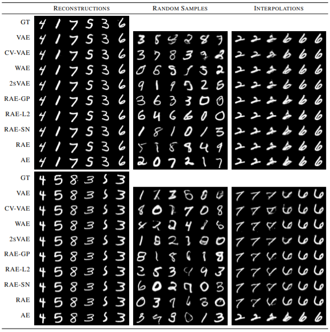
The following figure shows the qualitative evaluation for sample quality for VAEs, WAEs, and RAEs on MNIST. The first figure in the extreme left depicts the reconstructed samples (top row is ground truth) followed by randomly generated samples in the middle and spherical interpolations between two images at the extreme right.

These are remarkable results that show that the lack of an explicitly fixed structure on the latent space of the RAE does not impede interpolation quality.
Results:
Each model was trained and evaluated on the MNIST, CIFAR, and CELEBA datasets. Their performance across each metric and each dataset can be seen in figure 1. For the GMM metric and for each dataset, all RAE variants with regularization schemes outperform the baseline models. Furthermore, for [math]\displaystyle{ \mathcal{N} }[/math] the RAE regularized variants outperform the baseline models within the CIFAR and CELEBA datasets. This suggests RAE's can achieve competitive results for generated image quality when compared to existing VAE architectures.

Modelling Structured Objects
Overview
The authors evaluate RAEs ability to model the complex structured objects of molecules and arithmetic expressions. They adopt the exact architecture and experimental setting of the GrammarVAE (GVAE)[6] and replace its variational framework with that of an RAE's utilizing the Tikonov regularization (GRAE).
Metrics of Evaluation
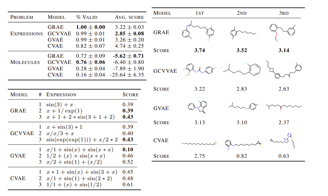
In this experiment, they are interested in traversing the learned latent space to generate samples for drug molecules and expressions. To evaluate the performance with respect to expressions, they consider [math]\displaystyle{ \log(1 + MSE) }[/math] between generated expressions and the true data. To evaluate the performance with respect to molecules they evaluate the water-octanol partition coefficient [math]\displaystyle{ \log(P) }[/math] where a higher value corresponds to a generated molecule having a more similar structure to that of a drug molecule. They compare the GRAEs performance on these metrics to those of the GVAE, the constant variance GVAE (GCVVAE), and the CharacterVAE (CVAE) [4] as seen in figure 2. Additionally, to assess the behavior within the latent space, they report the percentages of expressions and molecules with valid syntax's within the generated samples.
Results
Their results displayed in figure 2 show that the VRAE is competitive in its ability to generate samples of structured objects and even outperform the other models with respect to average score for generated expressions. It is notable that for generating molecules although they rank second in average score, it produces the highest percentage of syntactically valid molecules.

Conclusion
The authors provide empirical evidence that deterministic autoencoders are capable of learning a smooth latent space without the requirement of a prior distribution. This allows for the circumvention of drawbacks associated with the variational framework. By comparing the performance between VAEs and RAE's across the tasks of image and structured object sample generation the authors have demonstrated that RAEs are capable of producing comparable or better sample results.
Critiques
There is empirical evidence to support the sample quality of RAES is comparable to VAE’s. The Authors are inconclusive in determining how the different variants of regularization schemes affect the RAE’s performance as there was much variation between them for datasets. They do note they opted to use the L2 version in the structured objects experiment because it was the simplest to implement. There is also empirical evidence that using the ex-post density estimation when applied to existing VAE frameworks improves their sample quality as seen in the image generation experiment, this offers a plausible way to potentially improve existing VAE architectures. My Overall impression of the paper is they provided substantial evidence that a deterministic autoencoder can learn a latent space that is of comparable or better quality than that of a VAE. Although they observe favorable results for their RAE framework, it's still far from conclusive whether RAE will perform better in all data domains. A future comparison I would be interested in seeing is with VQ-VAE’s in the domain of sound generation.
Repository
The official repository for this paper is available at "official repository"
References
[1] Aaron van den Oord, Oriol Vinyals, et al. Neural discrete representation learning. In NeurIPS, 2017
[2] Bin Dai and David Wipf. Diagnosing and enhancing VAE models. In ICLR, 2019
[3] George Tucker, Andriy Mnih, Chris J Maddison, John Lawson, and Jascha Sohl-Dickstein. REBAR:low-variance, unbiased gradient estimates for discrete latent variable models. In NeurIPS, 2017
[4] Gómez-Bombarelli, Rafael, Jennifer N., Wei, David, Duvenaud, José Miguel, Hernández-Lobato, Benjamín, Sánchez-Lengeling, Dennis, Sheberla, Jorge, Aguilera-Iparraguirre, Timothy D., Hirzel, Ryan P., Adams, and Alán, Aspuru-Guzik. "Automatic Chemical Design Using a Data-Driven Continuous Representation of Molecules".ACS Central Science 4, no.2 (2018): 268–276.
[5] Ilya Tolstikhin, Olivier Bousquet, Sylvain Gelly, and Bernhard Scholkopf. Wasserstein autoencoders. In ICLR, 2017
[6] Matt J. Kusner, Brooks Paige, and José Miguel Hernández-Lobato. Grammar variational autoencoder. In ICML, 2017.
[7] Yuri Burda, Roger Grosse, and Ruslan Salakhutdinov. Importance weighted autoencoders. arXiv preprint arXiv:1509.00519, 2015.
[8] Diederik P Kingma and Max Welling. Auto-encoding variational Bayes. In ICLR, 2014.