learn what not to learn
Introduction
In reinforcement learning, it is often difficult for agent to learn when the action space is large. For a specific case that many actions are irrelevant, it is sometimes easier for the algorithm to learn which action not to take. The paper propose a new reinforcement learning approach for dealing with large action spaces by restricting the available actions in each state to a subset of the most likely ones. More specifically, it propose a system that learns the approximation of Q-function and concurrently learns to eliminate actions. The method need to utilize an external elimination signal which incorporates domain-specific prior knowledge. For example, in parser-based text games, the parser gives feedback regarding irrelevant actions after the action is played. (e.g., Player: "Climb the tree." Parser: "There are no trees to climb") Then a machine learning model can be trained to generalize to unseen states.
The paper focus mainly on tasks where both states and the actions are natural language. It introduces a novel deep reinforcement learning approach which has a DQN network and an Action Elimination Network(AEN), both using the CNN for NLP tasks. The AEN is trained to predict invalid actions, supervised by the elimination signal from the environment. Note that the core assumption is that it is easy to predict which actions are invalid or inferior in each state and leverage that information for control.
The text-based game called "Zork", which let player to interact with a virtual world through a text based interface, is tested by using the elimination framework. The AE algorithm has achieved faster learning rate than the baseline agents through eliminating irrelevant actions.
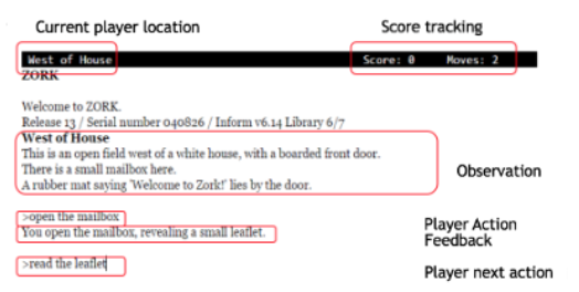
Below shows an example for the Zork interface:
All state and action are given in natural language. Input for the game contains more than a thousand possible actions in each state since player can type anything.
Related Work
Text-Based Games(TBG): The state of the environment in TBG is described by simple language. The player interacts with the environment with text command which respects a pre-defined grammar. A popular example is Zork which has been tested in the paper. TBG is a good research intersection of RL and NLP, it requires language understanding, long-term memory, planning, exploration, affordability extraction and common sense. It also often introduce stochastic dynamics to increase randomness.
Representations for TBG: Good word representation is necessary in order to learn control policies from texts. Previous work on TBG used pre-trained embeddings directly for control. other works combined pre-trained embedding with neural networks.
DRL with linear function approximation: DRL methods such as the DQN have achieved state-of-the-art results in a variety of challenging, high-dimensional domains. This is mainly because neural networks can learn rich domain representations for value function and policy. On the other hand, linear representation batch reinforcement learning methods are more stable and accurate, while feature engineering is necessary.
RL in Large Action Spaces: Prior work concentrated on factorizing the action space into binary subspace(Pazis and Parr, 2011; Dulac-Arnold et al., 2012; Lagoudakis and Parr, 2003), other works proposed to embed the discrete actions into a continuous space, then choose the nearest discrete action according to the optimal actions in the continuous space(Dulac-Arnold et al., 2015; Van Hasselt and Wiering, 2009). He et. al. (2015)extended DQN to unbounded(natural language) action spaces. Learning to eliminate actions was first mentioned by (Even-Dar, Mannor, and Mansour, 2003). They proposed to learn confidence intervals around the value function in each state. Lipton et al.(2016a) proposed to learn a classifier that detects hazardous state and then use it to shape the reward. Fulda et al.(2017) presented a method for affordability extraction via inner products of pre-trained word embedding.
Action Elimination
After executing an action, the agent observes a binary elimination signal e(s, a) to determine which actions not to take. It equals 1 if action a may be eliminated in state s (and 0 otherwise). The signal helps mitigating the problem of large discrete action spaces. We start with the following definitions:
Definition 1:
Valid state-action pairs with respect to an elimination signal are state action pairs which the elimination process should not eliminate.
Definition 2:
Admissible state-action pairs with respect to an elimination algorithm are state action pairs which the elimination algorithm does not eliminate.
Definition 3:
Action Elimination Q-learning is a Q-learning algorithm which updates only admissible state-action pairs and chooses the best action in the next state from its admissible actions. We allow the base Q-learning algorithm to be any algorithm that converges to [math]\displaystyle{ Q^* }[/math] with probability 1 after observing each state-action infinitely often.
The approach in the paper builds on the standard RL formulation. At each time step t, the agent observes state [math]\displaystyle{ s_t }[/math] and chooses a discrete action [math]\displaystyle{ a_t\in\{1,...,|A|\} }[/math]. Then the agent obtains a reward [math]\displaystyle{ r_t(s_t,a_t) }[/math] and next state [math]\displaystyle{ s_{t+1} }[/math]. The goal of the algorithm is to learn a policy [math]\displaystyle{ \pi(a|s) }[/math] which maximizes the expected future discount return [math]\displaystyle{ V^\pi(s)=E^\pi[\sum_{t=0}^{\infty}\gamma^tr(s_t,a_t)|s_0=s]. }[/math]After executing an action, the agent observes a binary elimination signal e(s,a), which equals to 1 if action a can be eliminated for state s, 0 otherwise.
Advantages of Action Elimination
The main advantages of action elimination is that it allows the agent to overcome some of the main difficulties in large action spaces which are Function Approximation and Sample Complexity.
Function approximation: Errors in the Q-function estimates may cause the learning algorithm to converge to a suboptimal policy, this phenomenon becomes more noticeable when the action space is large. Action elimination mitigate this effect by taking the max operator only on valid actions, thus, reducing potential overestimation. Besides, by ignoring the invalid actions, the function approximation can also learn a simpler mapping leading to faster convergence.
Sample complexity: The sample complexity measures the number of steps during learning, in which the policy is not [math]\displaystyle{ \epsilon }[/math]-optimal. The invalid action often returns no reward and doesn't change the state, (Lattimore and Hutter, 2012)resulting in an action gap of [math]\displaystyle{ \epsilon=(1-\gamma)V^*(s) }[/math], and this translates to [math]\displaystyle{ V^*(s)^{-2}(1-\gamma)^{-5}log(1/\delta) }[/math] wasted samples for learning each invalid state-action pair. Practically, elimination algorithm can eliminate these invalid actions and therefore speed up the learning process approximately by [math]\displaystyle{ A/A' }[/math].
Action elimination with contextual bandits
Let [math]\displaystyle{ x(s_t)\in R^d }[/math] be the feature representation of [math]\displaystyle{ s_t }[/math]. We assume that under this representation there exists a set of parameters [math]\displaystyle{ \theta_a^*\in R_d }[/math] such that the elimination signal in state [math]\displaystyle{ s_t }[/math] is [math]\displaystyle{ e_t(s_t,a) = \theta_a^Tx(s_t)+\eta_t }[/math], where [math]\displaystyle{ \Vert\theta_a^*\Vert_2\leq S }[/math]. [math]\displaystyle{ \eta_t }[/math] is an R-subgaussian random variable with zero mean that models additive noise to the elimination signal. When there is no noise in the elimination signal, R=0. Otherwise, [math]\displaystyle{ R\leq 1 }[/math] since the elimination signal is bounded in [0,1]. Assume the elimination signal satisfies: [math]\displaystyle{ 0\leq E[e_t(s_t,a)]\leq l }[/math] for any valid action and [math]\displaystyle{ u\leq E[e_t(s_t, a)]\leq 1 }[/math] for any invalid action. And [math]\displaystyle{ l\leq u }[/math]. Denote by [math]\displaystyle{ X_{t,a} }[/math] as the matrix whose rows are the observed state representation vectors in which action a was chosen, up to time t. [math]\displaystyle{ E_{t,a} }[/math] as the vector whose elements are the observed state representation elimination signals in which action a was chosen, up to time t. Denote the solution to the regularized linear regression [math]\displaystyle{ \Vert X_{t,a}\theta_{t,a}-E_{t,a}\Vert_2^2+\lambda\Vert \theta_{t,a}\Vert_2^2 }[/math] (for some [math]\displaystyle{ \lambda\gt 0 }[/math]) by [math]\displaystyle{ \hat{\theta}_{t,a}=\bar{V}_{t,a}^{-1}X_{t,a}^TE_{t,a} }[/math], where [math]\displaystyle{ \bar{V}_{t,a}=\lambda I + X_{t,a}^TX_{t,a} }[/math].
According to Theorem 2 in (Abbasi-Yadkori, Pal, and Szepesvari, 2011), [math]\displaystyle{ |\hat{\theta}_{t,a}^{T}x(s_t)-\theta_a^{*T}x(s_t)|\leq\sqrt{\beta_t(\delta)x(s_t)^T\bar{V}_{t,a}^{-1}x(s_t)} \forall t\gt 0 }[/math], where [math]\displaystyle{ \sqrt{\beta_t(\delta)}=R\sqrt{2log(det(\bar{V}_{t,a}^{1/2})det(\lambda I)^{-1/2}/\delta)}+\lambda^{1/2}S }[/math], with probability of at least [math]\displaystyle{ 1-\delta }[/math]. If [math]\displaystyle{ \forall s \Vert x(s)\Vert_2 \leq L }[/math], then [math]\displaystyle{ \beta_t }[/math] can be bounded by [math]\displaystyle{ \sqrt{\beta_t(\delta)} \leq R \sqrt{dlog(1+tL^2/\lambda/\delta)}+\lambda^{1/2}S }[/math]. Next, define [math]\displaystyle{ \tilde{\delta}=\delta/k }[/math] and bound this probability for all the actions. i.e., [math]\displaystyle{ \forall a,t\gt 0 }[/math]
[math]\displaystyle{ Pr(|\hat{\theta}_{t,a}^{T}x(s_t)-\theta_a^{*T}x(s_t)|\leq\sqrt{\beta_t(\delta)x(s_t)^T\bar{V}_{t,a}^{-1}x(s_t)}) \leq 1-\delta }[/math]
Recall that [math]\displaystyle{ E[e_t(s,a)]=\theta_a^{*T}x(s_t)\leq l }[/math] if a is a valid action. Then we can eliminate action a at state [math]\displaystyle{ s_t }[/math] if it satisfies:
[math]\displaystyle{ \hat{\theta}_{t,a}^{T}x(s_t)-\sqrt{\beta_t(\delta)x(s_t)^T\bar{V}_{t,a}^{-1}x(s_t)})\gt l }[/math]
with probability [math]\displaystyle{ 1-\delta }[/math] that we never eliminate any valid action. Note that [math]\displaystyle{ l, u }[/math] are not known. In practice, choosing [math]\displaystyle{ l }[/math] to be 0.5 should suffice.
Concurrent Learning
In fact, Q-learning and contextual bandit algorithms can learn simultaneously, resulting in the convergence of both algorithms, i.e., finding an optimal policy and a minimal valid action space.
If the elimination is done based on the concentration bounds of the linear contextual bandits, it can be ensured that Action Elimination Q-learning converges, as shown in Proposition 1.
Proposition 1:
Assume that all state action pairs (s,a) are visited infinitely often, unless eliminated according to [math]\displaystyle{ \hat{\theta}_{t-1,a}^Tx(s)-\sqrt{\beta_{t-1}(\tilde{\delta})x(s)^T\bar{V}_{t-1,a}^{-1}x(s))}\gt l }[/math]. Then, with a probability of at least [math]\displaystyle{ 1-\delta }[/math], action elimination Q-learning converges to the optimal Q-function for any valid state-action pairs. In addition, actions which should be eliminated are visited at most [math]\displaystyle{ T_{s,a}(t)\leq 4\beta_t/(u-l)^2 +1 }[/math] times.
Notice that when there is no noise in the elimination signal(R=0), we correctly eliminate actions with probability 1. so invalid actions will be sampled a finite number of times.
Method
The assumption that [math]\displaystyle{ e_t(s_t,a)=\theta_a^{*T}x(s_t)+\eta_t }[/math] might not hold when using raw features like word2vec. So the paper proposes to use the neural network's last layer as features. A practical challenge here is that the features must be fixed over time when used by the contextual bandit. So batch-updates framework(Levine et al., 2017;Riquelme, Tucker, and Snoek, 2018) is used, where a new contextual bandit model is learned for every few steps that uses the last layer activation of the AEN as features.
Architecture of action elimination framework
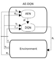
After taking action [math]\displaystyle{ a_t }[/math], the agent observes [math]\displaystyle{ (r_t,s_{t+1},e_t) }[/math]. The agent use it to learn two function approximation deep neural networks: A DQN and an AEN. AEN provides an admissible actions set [math]\displaystyle{ A' }[/math] to the DQN, which uses this set to decide how to act and learn. The architecture for both the AEN and DQN is an NLP CNN(100 convolutional filters for AEN and 500 for DQN, with three different 1D kernels of length (1,2,3)), based on(Kim, 2014). The state is represented as a sequence of words, composed of the game descriptor and the player's inventory. These are truncated or zero padded to a length of 50 descriptor + 15 inventory words and each word is embedded into continuous vectors using word2vec in [math]\displaystyle{ R^{300} }[/math]. The features of the last four states are then concatenated together such that the final state representations s are in [math]\displaystyle{ R^{78000} }[/math]. The AEN is trained to minimize the MSE loss, using the elimination signal as a label. The code, the Zork domain, and the implementation of the elimination signal can be found here.
Psuedocode of the Algorithm
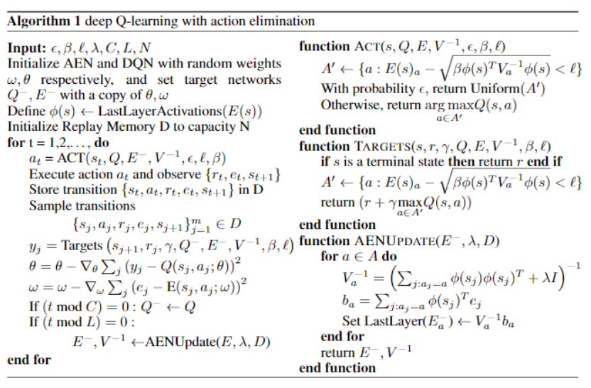
AE-DQN trains two networks: a DQN denoted by Q and an AEN denoted by E. The algorithm creates a linear contextual bandit model from it every L iterations with procedure AENUpdate(). This procedure uses the activations of the last hidden layer of E as features, which are then used to create a contextual linear bandit model.AENUpdate() then solved this model and plugin it into the target AEN. The contextual linear bandit model [math]\displaystyle{ (E^-,V) }[/math] is then used to eliminate actions via the ACT() and Target() functions. ACT() follows an [math]\displaystyle{ \epsilon }[/math]-greedy mechanism on the admissible actions set. For exploitation, it selects the action with highest Q-value by taking an argmax on Q-values among [math]\displaystyle{ A' }[/math]. For exploration, it selects an action uniformly from [math]\displaystyle{ A' }[/math]. The targets() procedure is estimating the value function by taking max over Q-values only among admissible actions, hence, reducing function approximation errors.
Experiment
Zork domain
The world of Zork presents a rich environment with a large state and action space. Zork players describe their actions using natural language instructions. For example, "open the mailbox". Then their actions were processed by a sophisticated natural language parser. Based on the results, the game presents the outcome of the action. The goal of Zork is to collect the Twenty Treasures of Zork and install them in the trophy case. Points that are generated from the game's scoring system are given to the agent as the reward. For example, the player gets the points when solving the puzzles. Placing all treasures in the trophy will get 350 points. The elimination signal is given in two forms, "wrong parse" flag, and text feedback "you cannot take that". These two signals are grouped together into a single binary signal which then provided to the algorithm.
Experiments begin with the two subdomains of Zork domains: Egg Quest and the Troll Quest. For these subdomains, an additional reward signal is provided to guide the agent towards solving specific tasks and make the results more visible. A reward of -1 is applied at every time step to encourage the agent to favor short paths. Each trajectory terminates is upon completing the quest or after T steps are taken. The discounted factor for training is [math]\displaystyle{ \gamma=0.8 }[/math] and [math]\displaystyle{ \gamma=1 }[/math] during evaluation. Also [math]\displaystyle{ \beta=0.5, l=0.6 }[/math] in all experiments.
Egg Quest
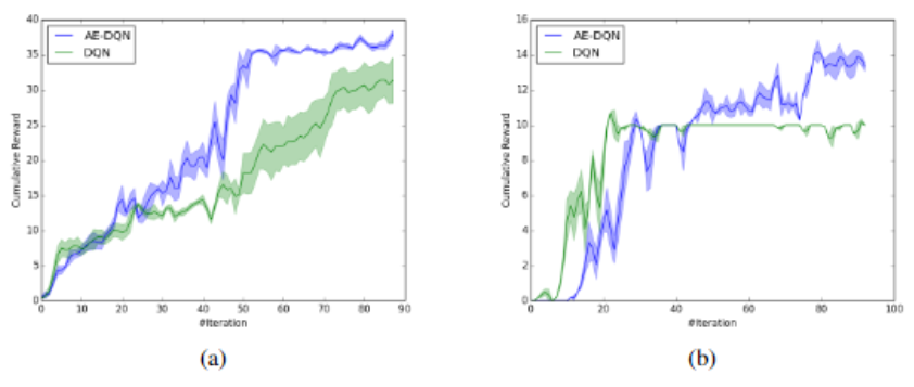
The goal for this quest is to find and open the jewel-encrusted egg hidden on a tree in the forest. The agent will get 100 points upon completing this task. For action space, there are 9 fixed actions for navigation, and a second subset which consisting [math]\displaystyle{ N_{Take} }[/math] actions for taking possible objects in the game. [math]\displaystyle{ N_{Take}=200 (set A_1), N_{Take}=300 (set A_2) }[/math] has been tested separately. AE-DQN (blue) and a vanilla DQN agent (green) has been tested in this quest.

Figure a) corresponds to the set [math]\displaystyle{ A_1 }[/math], with T=100, b) corresponds to the set [math]\displaystyle{ A_2 }[/math], with T=100, and c) corresponds to the set [math]\displaystyle{ A_2 }[/math], with T=200. Both agents has performed well on sets a and c. However the AE-DQN agent has learned much faster than the DQN on set b, which implies that action elimination is more robust to hyperparameter optimization when the action space is large. One important observation to note is that the three figures have different scales for the cumulative reward. While the AE-DQN outperformed the standard DQN in figure b, both models performed significantly better with the hyperparameter configuration in figure c.
Troll Quest
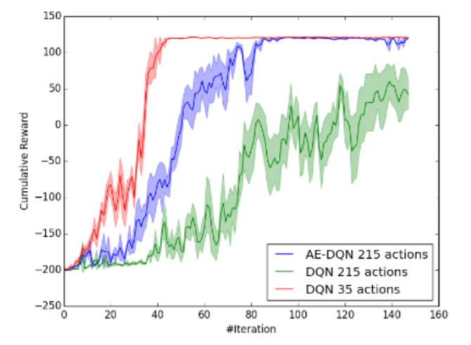
The goal of this quest is to find the troll. To do it the agent need to find the way to the house, use a lantern to expose the hidden entrance to the underworld. It will get 100 points upon achieving the goal. This quest is a larger problem than Egg Quest. The action set [math]\displaystyle{ A_1 }[/math] is 200 take actions and 15 necessary actions, 215 in total.
The red line above is an "optimal elimination" baseline which consists of only 35 actions(15 essential, and 20 relevant take actions). We can see that AE-DQN still outperforms DQN and its improvement over DQN is more significant in the Troll Quest than the Egg quest. Also, it achieves compatible performance to the "optimal elimination" baseline.
Open Zork
Lastly, the "Open Zork" domain has been tested which only the environment reward has been used. 1M steps has been trained. Each trajectory terminates after T=200 steps. Two action sets have been used:[math]\displaystyle{ A_3 }[/math], the "Minimal Zork" action set, which is the minimal set of actions (131) that is required to solve the game. [math]\displaystyle{ A_4 }[/math], the "Open Zork" action set (1227) which composed of {Verb, Object} tuples for all the verbs and objects in the game.
The above Figure shows the learning curve for both AE-DQN and DQN. We can see that AE-DQN (blue) still outperform the DQN (blue) in terms of speed and cumulative reward.
Conclusion
In this paper, the authors proposed a Deep Reinforcement Learning model for sub-optimal actions while performing Q-learning. Moreover, they showed that by eliminating actions, using linear contextual bandits with theoretical guarantees of convergence, the size of the action space is reduced, exploration is more effective, and learning is improved when tested on Zork, a text-based game.
For future work the authors aim to investigate more sophisticated architectures and tackle learning shared representations for elimination and control which may boost performance on both tasks.
They also hope to to investigate other mechanisms for action elimination, such as eliminating actions that result from low Q-values as in Even-Dar, Mannor, and Mansour, 2003.
Critique
The paper is not a significant algorithmic contribution and it merely adds an extra layer of complexity to the most famous DQN algorithm. All the experimental domains considered in the paper are discrete action problems that have so many actions that it could have been easily extended to a continuous action problem. In continuous action space there are several policy gradient based RL algorithms that have provided stronger performances. The authors should have ideally compared their methods to such algorithms like PPO or DRPO.
