End to end Active Object Tracking via Reinforcement Learning
Introduction
Object tracking has been a hot topic in recent years. It involves localization of an object in continuous video frames given an initial annotation in the first frame. The process normally consists of the following steps.
- Taking an initial set of object detections.
- Creating and assigning a unique ID for each of the initial detections.
- Tracking those objects as they move around in the video frames, maintaining the assignment of unique IDs.
There are two types of object tracking.
- Passive tracking
- Active tracking
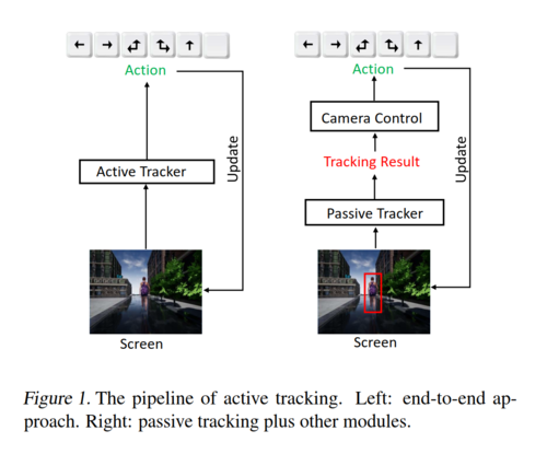
Passive tracking assumes that the object of interest is always in the image scene, meaning that there is no need for camera control during tracking. Although passive tracking is very useful and well-researched with existing works, it is not applicable in situations like tracking performed by a camera-mounted mobile robot or by a drone. On the other hand, active tracking involves two subtasks, including 1) Object Tracking and 2) Camera Control. It is difficult to jointly tune the pipeline between these two separate subtasks. Object Tracking may require human efforts for bounding box labeling. In addition, Camera Control is non-trivial, which can lead to many expensive trial-and-errors in the real world.
To address these challenges, this paper presents an end-to-end active tracking solution via deep reinforcement learning. More specifically, the ConvNet-LSTM network takes raw video frames as input and outputs camera movement actions. The virtual environment is used to simulate active tracking. In a virtual environment, an agent (i.e. the tracker) observes a state (a visual frame) from a first-person perspective and takes an action. Then, the environment returns the updated state (next visual frame). A3C, a modern Reinforcement Learning algorithm, is adopted to train the agent, where a customized reward function is designed to encourage the agent to be closely following the object. Environment augmentation technique is used to boost the tracker’s generalization ability. The tracker trained in the virtual environment is then tested on a real-world video dataset to assess the generalizability of the model. A video of the first version of this paper is available here[1].
Intuition
As in the case of the state of the art models, if the action module and the object tracking module are completely different, it is extremely difficult to train one or the other as it is impossible to know which is causing the error that is being observed at the end of the episode. The function of both these modules are the same at a high level as both are aiming for efficient navigation. So it makes sense to have a joint module that consists of both the observation and the action taking submodules. Now we can train the entire system together as the error needs to be propagated to the whole system. This is in line with the common practice in Deep Reinforcement Learning where the CNNs used to extract features in the case of Atari games are combined with the Q networks (in the case of DQN). The training of these CNN happens concurrently with the Q feedforward networks where the error function is the difference between the observed Q value and the target Q values.
Related Work
In the domain of object tracking, there are both active and passive approaches. The below summarize the advance passive object tracking approaches:
1) Subspace learning was adopted to update the appearance model of an object.
- Formerly, object tracking algorithms employ a fixed appearance model. Consequently, they often perform poorly when the target object changes in appearance or illumination. To overcome this problem, Ross et al. 2008 introduce a novel tracking method that incrementally adapts the appearance model according to new observations made during tracking [2].
2) Multiple instance learning was employed to track an object.
- Many researchers have shown that a tracking algorithm can achieve better performance by employing adaptive appearance models capable of separating an object from its background. However, the discriminative classifier in those models is often difficult to update. So, Babenko et al. 2009 introduce a novel algorithm that updates its appearance model using a “bag” of positive and negative examples. Subsequently, they show that tracking algorithms using weaker classifiers can still obtain superior performance [3].
3) Correlation filter based object tracking has achieved success in real-time object tracking.
- Correlation filter based object tracking algorithms attempt to “model the appearance of an object using filters”. At each frame, a small tracking window representing the target object is produced, and the tracker will correlate the windows over the image sequences, thus achieving object tracking. Bolme et al. 2010 validate this concept by creating a novel object tracking algorithm using an adaptive correlation filter called Minimum Output Sum of Squared Error (MOSSE) filter [4].
4) Structured Output predicted was used to constrain object tracking and avoiding converting positions to labels of training samples.
- Hare et al. 2016 argue the “sliding-window” approach use by popular object tracking algorithms is flawed because “the objective of the classifier (predicting labels for sliding-windows) is decoupled from the objective of the tracker (estimating object position).” Instead, they introduce a novel algorithm that uses “a kernelized structured output support vector machine (SVM) to avoid the need for intermediate classification”. Subsequently, they show the approach outperforms traditional trackers in various benchmarks [5].
5) Tracking, learning, and Detection were integrated into one framework for long-term tracking, where a detection module was used to re-initialize the tracker once a missing object reappears.
- Long-Term Tracking is the task to recognize and track an object as it “moves in and out of a camera’s field of view”. This task is made difficult by problems such as an object reappearing into the scene and changing its appearance, scale, or illumination. Kalal et al. 2012 proposed a unified tracking framework (TLD) that accomplishes long-term tracking by “decomposing the task into tracking, learning, and detection”. Specifically, “the tracker follows an object from frame-to-frame; the detector localizes the object’s appearances; and, the learner improves the detector by learning from errors.” Altogether, the TLD framework outperforms previous state-of-arts tracking approaches [6].
6) Deep learning models like stacked autoencoder have been used to learn good representations for object tracking.
- In recent year, Deep Learning approaches are gaining prominence in the field of object tracking. For example, Wang et al. 2013 obtain outstanding results using a deep-learning based algorithm that combines offline feature extraction and online tracking using stacked denoising autoencoders. Whereas, Wang et al. 2016 introduced a sequential training convolutional network that can efficiently transfer offline learned features for online visual tracking applications.
For the active approaches, camera control and object tracking were considered as separate components. These approaches are difficult to tune. This paper tackles object tracking and camera control simultaneously in an end to end manner and is easy to tune.
In the domain of domain of deep reinforcement learning, recent algorithms have achieved advanced gameplay in games like GO and Atari games. They have also been used in computer vision tasks like object localization, region proposal, and visual tracking. All advancements pertain to passive tracking but this paper focusses on active tracking using Deep RL, which has never been tried before.
Approach
Virtual tracking scenes are generated for both training and testing. An Asynchronous Actor-Critic Agents (A3C) model was used to train the tracker. For efficient training, data augmentation techniques and a customized reward function were used. An RGB screen frame of the first-person perspective was chosen as the state for the study. The tracker observes a visual state and takes one action [math]\displaystyle{ a_t }[/math] from the following set of 6 actions.
\[A = \{\text{turn-left}, \text{turn-right}, \text{turn-left-and-move-forward},\\ \text{turn-right-and-move-forward}, \text{move-forward}, \text{no-op}\}\]
The action is processed by the environment, which returns to the agent the current reward as well as the updated screen frame [math]\displaystyle{ (r_t, s_{t+1}) }[/math].
Tracking Scenarios
It is impossible to train the desired end-to-end active tracker in real-world scenarios. Therefore, The following two Virtual environment engines are used for the simulated training.
ViZDoom
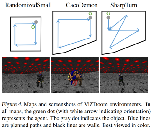
ViZDoom[2] (Kempka et al., 2016; ViZ) is an RL research platform based on a 3D FPS video game called Doom. In ViZDoom, the game engine corresponds to the environment, while the video game player corresponds to the agent. The agent receives from the environment a state and a reward at each time step. In this study, customized ViZDoom maps are used. (see Fig. 4) composed of an object (a monster) and background (ceiling, floor, and wall). The monster walks along a pre-specified path programmed by the ACS script (Kempka et al., 2016), and the goal is to train the agent, i.e., the tracker, to follow closely the object.
Unreal Engine
Though convenient for research, ViZDoom does not provide realistic scenarios. To this end, Unreal Engine (UE) is adopted to construct nearly real-world environments. UE is a popular game engine and has a broad influence in the game industry. It provides realistic scenarios which can mimic real-world scenes. UnrealCV (Qiu et al., 2017) is employed in this study, which provides convenient APIs, along with a wrapper (Zhong et al., 2017) compatible with OpenAI Gym (Brockman et al., 2016), for interactions between RL algorithms and the environments constructed based on UE.
A3C Algorithm
This paper employs the Asynchronous Actor-Critic Agents (A3C) algorithm for training the tracker. At time step t, [math]\displaystyle{ s_{t} }[/math] denotes the observed state corresponding to the raw RGB frame. The action set is denoted by A of size K = |A|. An action, [math]\displaystyle{ a_{t} }[/math] ∈ A, is drawn from a policy function distribution: \[a_{t}\sim \pi\left ( . | s_{t} \right ) \in \mathbb{R}^{k} \] This is referred to as actor. The environment then returns a reward [math]\displaystyle{ r_{t} \in \mathbb{R} }[/math] , according to a reward function [math]\displaystyle{ r_{t} = g(s_{t}) }[/math] . The updated state [math]\displaystyle{ s_{t+1} }[/math] at next time step t+1 is subject to a certain but unknown state transition function [math]\displaystyle{ s_{t+1} = f(s_{t}, a_{t}) }[/math], governed by the environment. Trace consisting of a sequence of triplets can be observed. \[\tau = \{\ldots, (s_{t}, a_{t}, r_{t}) , (s_{t+1}, a_{t+1}, r_{t+1}) , \ldots \}\] Meanwhile, [math]\displaystyle{ V(s_{t}) \in \mathbb{R} }[/math] denotes the expected accumulated reward in the future given state [math]\displaystyle{ s_{t} }[/math] (referred to as Critic). The policy function [math]\displaystyle{ \pi(.) }[/math] and the value function [math]\displaystyle{ V (·) }[/math] are then jointly modeled by a neural network. Rewriting these as [math]\displaystyle{ \pi(.|s_{t};\theta) }[/math] and [math]\displaystyle{ V(s_{t};{\theta}') }[/math] with parameters [math]\displaystyle{ \theta }[/math] and [math]\displaystyle{ {\theta}' }[/math] respectively. The parameters are learned over trace [math]\displaystyle{ \tau }[/math] by simultaneous stochastic policy gradient and value function regression.
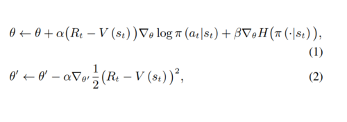
Where [math]\displaystyle{ R_{t} = \sum_{{t}'=t}^{t+T-1} \gamma^{{t}'-t}r_{{t}'} }[/math] is a discounted sum of future rewards up to [math]\displaystyle{ T }[/math] time steps with a factor [math]\displaystyle{ 0 \lt \gamma \leq 1, \alpha }[/math] is the learning rate, [math]\displaystyle{ H (·) }[/math] is an entropy regularizer, and [math]\displaystyle{ \beta }[/math] is the regularizer factor.
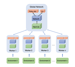
This is a multi-threaded training process where each thread maintains an independent environment-agent interaction. Nevertheless, the network parameters are shared among threads and are updated asynchronously every T-time step using eq 1 in a lock-free manner in each thread.
Network Architecture
The tracker is a ConvNet-LSTM neural network as shown in Fig. 2, where the architecture specification is given in the following table. The FC6 and FC1 correspond to the 6-action policy [math]\displaystyle{ \pi (·|s_{t}) }[/math] and the value [math]\displaystyle{ V (s_{t}) }[/math], respectively. The screen is resized to 84 × 84 × 3 RGB images as the network input.


Reward Function
The reward function utilizes a two-dimensional local coordinate system (S). The x-axis points from the agent’s left shoulder to right shoulder and the y-axis points perpendicular to the x-axis and points to the agent’s front. The origin is where is the agent is. System S is parallel to the floor. The object’s local coordinate (x,y) and orientation a with regard to the system S. The reward function is defined as follows.

Where A>0, c>0, d>0 and λ>0 are tuning parameters. The reward equation states that the maximum reward A is achieved when the object stands perfectly in front of the agent with distanced and exhibits no rotation.
Environment Augmentation
To make the tracker generalize well, an environment augmentation technique is proposed for both virtual environments.
For ViZDoom, (x,y, a) define the system state. For augmentation the initial system state is perturbed N times by editing the map with ACS script (Kempka et al., 2016), yielding a set of environments with varied initial positions and orientations [math]\displaystyle{ \{x_{i},y_{i},a_{i}\}_{i=1}^{N} }[/math]. Further flipping left-right the screen frame (and accordingly the left-right action) is allowed. As a result, 2N environments are obtained out of one environment. During A3C training, one of the 2N environments is randomly sampled at the beginning of every episode. This makes the generalization ability of the tracker be improved.
For UE, an environment with a character/target following a fixed path is constructed. To augment the environment, random background objects are chosen and making them invisible. Simultaneously, every episode starts from the position, where the agent fails at the last episode. This makes the environment and starting point different from episode to episode, so the variations of the environment during training are augmented.
Experimental Settings
Environment Setup
A set of environments are produced for both training and testing. For ViZDoom, a training map as in Fig. 4, left column is adopted. This map is then augmented with N = 21, leading to 42 environments that can be sampled from during training. For testing, 9 maps are made, some of which are shown in Fig. 4, middle and right columns. In all maps, the path of the target is pre-specified, indicated by the blue lines. However, it is worth noting that the object does not strictly follow the planned path. Instead, it sometimes randomly moves in a “zig-zag” way during the course, which is a built-in game engine behavior. This poses an additional difficulty to the tracking problem. For UE, an environment named Square with random invisible background objects is generated and a target named Stefani walking along a fixed path for training. For testing, another four environments named as Square1StefaniPath1 (S1SP1), Square1MalcomPath1 (S1MP1), Square1StefaniPath2 (S1SP2), and Square2MalcomPath2 (S2MP2) are made. As shown in Fig. 5, Square1 and Square2 are two different maps, Stefani and Malcom are two characters/targets, and Path1 and Path2 are different paths. Note that, the training environment Square is generated by hiding some background objects in Square1. For both ViZDoom and UE, an episode is terminated when either the accumulated reward drops below a threshold or the episode length reaches a maximum number. In these experiments, the reward threshold is set as -450 and the maximum length as 3000, respectively.
Metric
Two metrics are employed for the experiments. Accumulated Reward (AR) and Episode Length (EL). AR is like Precision in the conventional tracking literature. An AR that is too small leads to termination of the episode because it essentially means a failure of tracking. EL roughly measures the duration of good tracking and is analogous to the metric Successfully Tracked Frames in conventional tracking applications. The theoretical maximum for both AR and EL is 3000 when letting A = 1.0 in the reward function (because of the termination criterion).
Results
Two training protocols were followed namely RandomizedEnv(with augmentation) and SingleEnv(without the augmentation technique). However, only the results for RandomizedEnv are reported in the paper. There is only one table specifying the result from SingleEnv training which shows that it performs worse than the RandomizedEnv training. Compared to RandomizedEnv, SingleEnv does not exploit the capacity of the network better. The variability in the test results is very high for the non-augmented training case.

The testing environments results are reported in Tab. 2. These are 8 more challenging test environments that present different target appearances, different backgrounds, more varied paths and distracting targets comparing to the training environment.
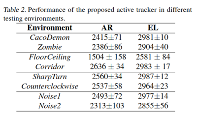
Following are the findings from the testing results: 1. The tracker generalizes well in the case of target appearance changing (Zombie, Cacodemon). 2. The tracker is insensitive to background variations such as changing the ceiling and floor (FloorCeiling) or placing additional walls in the map (Corridor). 3. The tracker does not lose a target even when the target takes several sharp turns (SharpTurn). Note that in conventional tracking, the target is commonly assumed to move smoothly. 4. The tracker is insensitive to a distracting object (Noise1) even when the “bait” is very close to the path (Noise2).
The proposed tracker is compared against several of the conventional trackers with PID like module for camera control to simulate active tracking. The results are displayed in Tab. 3.
The camera control module is implemented such that in the first frame, a manual bounding box must be given to indicate the object to be tracked. For each subsequent frame, the passive tracker then predicts a bounding box which is passed to the Camera Control module. A comparison is made between the two subsequent bounding boxes as per the algorithm and action decision is made. The results show that the proposed solution outperforms the simulated active tracker. The simulated trackers lost their targets soon. The Meanshift tracker works well when there is no camera shift between continuous frames. Both KCF and Correlation trackers seem not capable of handling such a large camera shift, so they do not work as well as the case in passive tracking. The MIL tracker works reasonably in the active case, while it easily drifts when the object turns suddenly.
Testing in the UE environment is tabulated in Table 5. Four different environments are tested and based on the long-term TLD tracker.
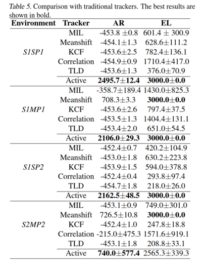
1. Comparison between S1SP1 and S1MP1 shows that the tracker generalizes well even when the model is trained with target Stefani, revealing that it does not overfit to a specialized appearance. 2. The active tracker performs well when changing the path (S1SP1 versus S1SP2), demonstrating that it does not act by memorizing specialized path. 3. When the map is changed, target, and path at the same time (S2MP2), though the tracker could not seize the target as accurately as in previous environments (the AR value drops), it can still track objects robustly (comparable EL value as in previous environments), proving its superior generalization potential. 4. In most cases, the proposed tracker outperforms the simulated active tracker or achieves comparable results if it is not the best. The results of the simulated active tracker also suggest that it is difficult to tune a unified camera-control module for them, even when a long-term tracker is adopted (see the results of TLD).
Real world active tracking: To test and evaluate the tracker in real-world scenarios, the network trained on UE environment is tested on a few videos from the VOT dataset.
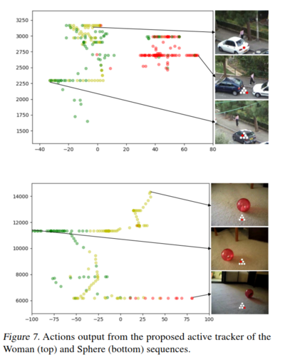
Fig. 7 shows the output actions for two video clips named Woman and Sphere, respectively. The horizontal axis indicates the position of the target in the image, with a positive (negative) value meaning that a target in the right (left) part. The vertical axis indicates the size of the target, i.e., the area of the ground truth bounding box. Green and red dots indicate turn-left/turn-left-and-move-forward and turn-right/turn-right-and-move-forward actions, respectively. Yellow dots represent No-op action. As the figure shows, 1) When the target resides in the right (left) side, the tracker tends to turn right (left), trying to move the camera to “pull” the target to the center. 2) When the target size becomes bigger, which probably indicates that the tracker is too close to the target, the tracker outputs no-op actions more often, intending to stop and wait for the target to move farther.
Video Link to the experimental results can be found below: Video Demonstration of the Results
Supplementary Material for Further Experiments: Additional PDF and Video
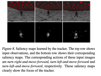
Action Saliency Map: An input frame is fed into the tracker and forwarded to output the policy function. An action will be sampled subsequently. Then the gradient of this action is propagated backwards to the input layer, the saliency map is generated. According to the saliency map, how the input image affects the tracker's action can be observed. Fig. 8 shows the tracker indeed learns how to find the target, which improves the performance of the model.
Conclusion
In the paper, an end-to-end active tracker via deep reinforcement learning is proposed. Unlike conventional passive trackers, the proposed tracker is trained in simulators, saving the efforts of human labeling or trial-and-errors in real-world. It shows good generalization to unseen environments. The tracking ability can potentially transfer to real-world scenarios.
Critique
The paper presents a solution for active tracking using reinforcement learning. A ConvNet-LSTM network has been adopted. Environment augmentation has been proposed for training the network. The tracker trained using environment augmentation performs better than the one trained without it. This is true in both the ViZDoom and UE environment. The reward function looks intuitive for the task at hand which is object tracking. The virtual environment ViZDoom though used for training and testing, seems to have little or no generalization ability in real-world scenarios. The maps in ViZDoom itself are very simple. The comparison presented in the paper for the ViZDoom testing with changes in the environmental parameters look positive, but the relatively simple nature of the environment needs to be considered while looking at these results. Also, when the floor is replaced by the ceiling, the tracker performs worst in comparison to the other cases in the table, which seems to indicate that the floor and ceiling parameters are somewhat over-fitted in the model. The tracker trained in UE environment is tested against simulated trackers. The results show that the proposed solution performs better than the simulated trackers. However, since the trackers are simulated using the camera control algorithm written for this specific comparison, further testing is required for benchmarking. The real-world challenges of intensity variation, camera details, control signals through beyond the scope of the current paper, still need to be considered while discussing the generalization ability of the model to real-world scenarios. For example, the current action space includes only six discrete actions, which are inadequate for deployment in the real world because the tracker cannot adapt to the different moving speed of the target. It is also believed that training the tracker in UE simulator alone is sufficient for a successful real-world deployment. It is better to randomize more aspects of the environment during training, including the texture of each mesh, the illumination condition of the scene, the trajectory of the target as well as the speed of the target. The results on the real-world videos show a positive result towards the generalization ability of the models in real-world settings. The overall approach presented in the paper is intuitive and the results look promising.
Future Work
The authors did some future work for this paper in several ways. Basically, they implemented a successful robot. Moreover, they enhanced the system to deal with the virtual-to-real gap [1]. Specifically, 1) more advanced environment augmentation techniques have been proposed to boost the environment diversity, which improves the transferability tailored to the real world. 2) A more appropriate action space compared with the conference paper is developed, and using a continuous action space for active tracking is investigated. 3) A mapping from the neural network prediction to the robot control signal is established so as to successfully deliver the end-to-end tracking.
References
1 W. Luo, P. Sun, F. Zhong, W. Liu, T. Zhang, and Y. Wang, “End-to-end Active Object Tracking and Its Real-world Deployment via Reinforcement Learning”.
[2] Ross, David A, Lim, Jongwoo, Lin, Ruei-Sung, and Yang, Ming- Hsuan. Incremental learning for robust visual tracking. International Journal of Computer Vision, 77(1-3):125–141, 2008.
[3] Babenko, Boris, Yang, Ming-Hsuan, and Belongie, Serge. Visual tracking with online multiple instance learning. In The IEEE Conference on Computer Vision and Pattern Recognition, pp. 983–990, 2009.
[4] Bolme, David S, Beveridge, J Ross, Draper, Bruce A, and Lui, Yui Man. Visual object tracking using adaptive correlation filters. In The IEEE Conference on Computer Vision and Pattern Recognition, pp. 2544–2550, 2010.
[5] Hare, Sam, Golodetz, Stuart, Saffari, Amir, Vineet, Vibhav, Cheng, Ming-Ming, Hicks, Stephen L, and Torr, Philip HS. Struck: Structured output tracking with kernels. IEEE Transactions on Pattern Analysis and Machine Intelligence, 38(10):2096–2109, 2016.
[6] Kalal, Zdenek, Mikolajczyk, Krystian, and Matas, Jiri. Tracking- learning-detection. IEEE Transactions on Pattern Analysis and Machine Intelligence, 34(7):1409–1422, 2012.
[7] Wang, Naiyan and Yeung, Dit-Yan. Learning a deep compact image representation for visual tracking. In Advances in Neural Information Processing Systems, pp. 809–817, 2013.
[8] Wang, Lijun, Ouyang, Wanli, Wang, Xiaogang, and Lu, Huchuan. Stct: Sequentially training convolutional networks for visual tracking. In The IEEE Conference on Computer Vision and Pattern Recognition, pp. 1373–1381, 2016.