STAT946F17/Conditional Image Generation with PixelCNN Decoders
Introduction
This work is based on the widely used PixelCNN and PixelRNN, introduced by Oord et al. in [1]. PixelRNN is a deep neural network that sequentially predicts the pixels in an image along the two spatial dimensions. You can find a nice video on this topic here, and also you can find more details here. From the previous work, the authors observed that PixelRNN performed better than PixelCNN, however, PixelCNN was faster to compute as you can parallelize the training process. In this work, Oord et al. [2] introduced a Gated PixelCNN, which is a convolutional variant of the PixelRNN model, based on PixelCNN. In particular, the Gated PixelCNN uses explicit probability densities to generate new images using autoregressive connections to model images through pixel-by-pixel computation by decomposing the joint image distribution as a product of conditionals [6]. The Gated PixelCNN is an improvement over the PixelCNN by removing the "blindspot" problem, and to yield a better performance, the authors replaced the ReLU units with sigmoid and tanh activation function. The proposed Gated PixelCNN combines the strength of both PixelRNN and PixelCNN - that is by matching the log-likelihood of PixelRNN on both CIFAR and ImageNet along with the quicker computational time presented by the PixelCNN [9]. Moreover, the authors introduced a conditional Gated PixelCNN variant (called Conditional PixelCNN) which has the ability to generate images based on class labels, tags, as well as latent embedding to create new image density models. These embeddings capture high level information of an image to generate a large variety of images with similar features; for instance, the authors can generate different poses of a person based on a single image by conditioning on a one-hot encoding of the class. This approach provided insight into the invariances of the embeddings which enabled the authors to generate different poses of the same person based on a single image. Finally, the authors also presented a PixelCNN Auto-encoder variant which essentially replaces the deconvolutional decoder with the PixelCNN.
The followings present a short comparison between different generative models.

| VAE | GAN | Autoregressive Models | |
|---|---|---|---|
| Pros | Efficient inference with approximate latent variables. | GAN can generate sharp image; There is no need for any Markov chain or approx networks during sampling. | The model is very simple and training process is stable. It currently gives the best log likelihood, which is tractable. |
| Cons | generated samples tend to be blurry. | difficult to optimize due to unstable training dynamics. | relatively inefficient during sampling |
Gated PixelCNN
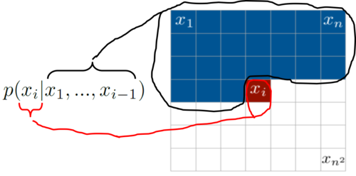
Pixel-by-pixel is a simple generative method wherein given an image of dimension $x_{n^2}$, we iterate, employ feedback and capture pixel densities from every pixel to predict our "unknown" pixel density $x_i$. To do this, the traditional PixelCNNs and PixelRNNs adopted the joint distribution p(x), wherein the pixels of a given image is the product of the conditional distributions. Hence, as depicted in Equation 1, the authors employ autoregressive models which simply use chain rule to compute the joint distribution. The ordering of the pixel dependencies is in raster scan order: row by row and pixel by pixel within every row. Every pixel, therefore, depends on all the pixels above and to the left of it, and not on any of other pixels ( So the very first pixel is independent, second depend on first, third depends on first and second and so on). Basically, you just model your image as a sequence of points where each pixel depends linearly on previous ones. Equation 1 depicts the joint distribution where x_i is a single pixel:
$$p(x) = \prod\limits_{i=1}^{n^2} p(x_i | x_1, ..., x_{i-1})$$
where $p(x)$ is the generated image, $n^2$ is the number of pixels, and $p(x_i | x_1, ..., x_{i-1})$ is the probability of the $i$th pixel which depends on the values of all previous pixels. It is important to note that $p(x_0, x_1, ..., x_{n^2})$ is the joint probability based on the chain rule - which is a product of all conditional distributions $p(x_0) \times p(x_1|x_0) \times p(x_2|x_1, x_0)$ and so on. Figure 1 provides a pictorial understanding of the joint distribution which displays that the pixels are computed pixel-by-pixel for every row, and the forthcoming pixel depends on the pixels values above and to the left of the pixel in concern.
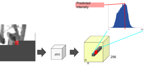
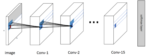
Therefore, to predict the pixel intensity value (i.e. the highest probable index from 0 to 255), a softmax layer is used for every pixel towards the end of the PixelCNN. Figure 2 [7] illustrates how to predict (generate) a single pixel value.
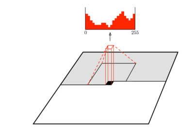
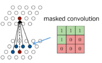
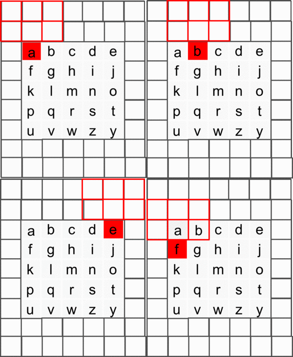
To reivew, the PixelCNN aims to map a neighborhood of pixels to the prediction for the next pixel. That is, to generate pixel $x_i$ the model can only condition on the previously generated pixels $x_1 , ..., x_{i−1}$; so every conditional distribution is modeled by a convolutional neural network. For instance, given a $5\times5$ image (let's represent each pixel as an alphabet and zero-padded), and we have a filter of dimension $3\times3$ that slides over the image which multiplies each element and sums them together to produce a single response. However, we cannot use this filter because pixel $a$ should not know the pixel intensities for $b,f,g$ (future pixel values). To counter this issue, the authors use a mask on top of the filter to only choose prior pixels and zeroing the future pixels to negate them from calculation - depicted in Figure 3 [7]. Hence, to make sure the CNN can only use information about pixels above and to the left of the current pixel, the filters of the convolution are masked - that means the model cannot read pixels below (or strictly to the right) of the current pixel to make its predictions [3].
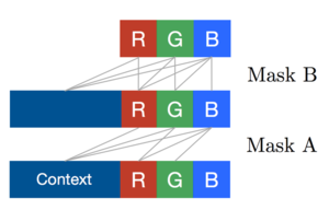
Hence, for each pixel, there are three colour channels (R, G, B) which are modeled successively, with B conditioned on (R, G), and G conditioned on R [8]. This is achieved by splitting the feature maps at every layer of the network into three and adjusting the center values of the mask tensors, as depicted in Figure 5 [8]. The 256 possible values for each colour channel are then modeled using a softmax.
Now, from Figure 6, notice that as the filter with the mask slides across the image, pixel $f$ does not take pixels $c, d, e$ into consideration (breaking the conditional dependency) - this is where we encounter the "blind spot" problem.
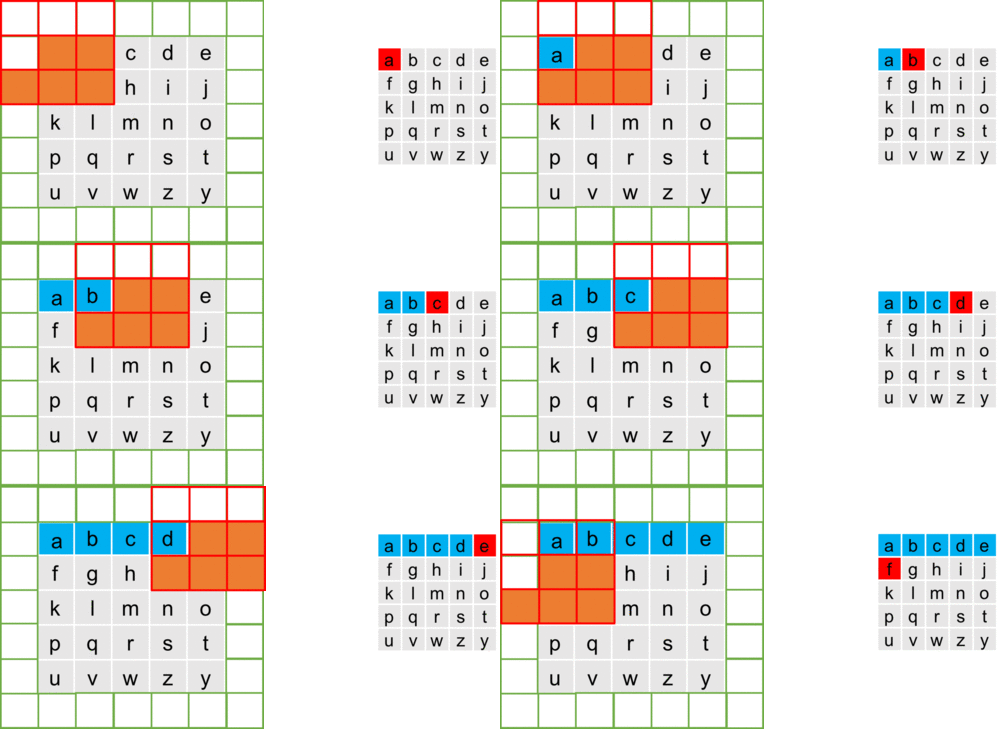
It is evident that the progressive growth of the receptive field of the masked kernel over the image disregards a significant portion of the image. For instance, when using a 3x3 filter, roughly quarter of the receptive field is covered by the "blind spot", meaning that the pixel contents are ignored in that region. In order to address the blind spot, the authors use two filters (horizontal and vertical stacks) in conjunction to allow for capturing the whole receptive field, depicted in Figure{vh_stack}. In particular, the horizontal stack conditions the current row, and the vertical stack conditions all the rows above the current pixel. It is observed that the vertical stack, which does not have any masking, allows the receptive field to grow in a rectangular fashion without any blind spot. Thereafter, the outputs of both the stacks, per-layer, is combined to form the output. Hence, every layer in the horizontal stack takes an input which is the output of the previous layer as well as that of the vertical stack. By splitting the convolution into two different operations enables the model to access all pixels prior to the pixel of interest.

Horizontal Stack
For the horizontal stack (in purple for Figure 7), the convolution operation conditions only on the current row, so it has access to left pixels. In essence, we take a $1 \times n//2+1$ convolution with shift (pad and crop) rather than $1\times n$ masked convolution. So, we perform convolution on the row with a kernel of width 2 pixels (instead of 3) from which the output is padded and cropped such that the image shape stays the same. Hence, the image convolves with kernel width of 2 and without masks.

Figure 8 [3] shows that the last pixel from the output (just before ‘Crop here’ line) does not hold information from last input sample (which is the dashed line).
Vertical Stack
Vertical stack (blue) has access to all top pixels. The vertical stack is of kernel size $n/2 + 1 \times n$ with the input image being padded with another row in the top and bottom. Thereafter, we perform the convolution operation, and crop the image to force the predicted pixel to be dependent on the upper pixels only (i.e. to preserve the spatial dimensions)[3]. Since the vertical filter does not contain any "future" pixel values, only upper pixel values, no masking is incorporated as no target pixel is touched. However, the computed pixel from the vertical stack yields information from top pixels and sends that info to horizontal stack (which supposedly eliminates the "blindspot problem").
From Figure 9 it is evident that the image is padded (left) with kernel height zeros, then convolution operation is performed from which we crop the output so that rows are shifted by one with respect to the input image. Hence, it is noticeable that the first row of output does not depend on first (real, non-padded) input row. Also, the second row of output only depends on the first input row - which is the desired behaviour.
Gated block
The PixelRNNs are observed to perform better than the traditional PixelCNN for generating new images. This is because the spatial LSTM layers in the PixelRNN allows for every layer in the network to access the entire neighborhood of previous pixels. The PixelCNN, however, only takes into consideration the neighborhood region and the depth of the convolution layers to make its predictions [4]. Another advantage for the PixelRNN is that this network contains multiplicative units (in the form of the LSTM gates), which may help it to model more complex interactions [3]. To address the benefits of PixelRNN and append it onto the newly proposed Gated PixelCNN, the authors replaced the rectified linear units between the masked convolutions with the following custom-made gated activation function which alleviates the problem, depicted in Equation 2:
$$y = tanh(W_{k,f} \ast x) \odot \sigma(W_{k,g} \ast x)$$
- $*$ is the convolutional operator.
- $\odot$ is the element-wise product.
- $\sigma$ is the sigmoid non-linearity
- $k$ is the number of the layer
- $tanh(W_{k,f} \ast x)$ is a classical convolution with tanh activation function.
- $sigmoid(\sigma(W_{k,g} \ast x)$ are the gate values (0 = gate closed, 1 = gate open).
- $W_{k,f}$ and $W_{k,g}$ are learned weights.
- $f, g$ are the different feature maps
This function is the key ingredient that cultivates the Gated PixelCNN model.
Figure 10 provides a pictorial illustration of a single layer in the Gated PixelCNN architecture; wherein the vertical stack contributes to the horizontal stack with the $1\times1$ convolution - going the other way would break the conditional distribution. In other words, the horizontal and vertical stacks are sort of independent, wherein vertical stack should not access any information horizontal stack has - otherwise it will have access to pixels it shouldn’t see. However, the vertical stack can be connected to vertical as it predicts pixel following those in the vertical stack. In particular, the convolution operations are shown in green (which are masked), element-wise multiplications and additions are shown in red. The convolutions with $W_f$ and $W_g$ are not combined into a single operation (which is essentially the masked convolution) to increase parallelization shown in blue. The parallelization now splits the $2p$ features maps into two groups of $p$. Finally, the authors also use the residual connection in the horizontal stack. Moreover, the $(n \times 1)$ and $(n \times n)$ are the masked convolutions which can also be implemented as $([n/2] \times 1)$ and $([n/2] \times n)$ which are convolutions followed by a shift in pixels by padding and cropping to get the original dimension of the image.
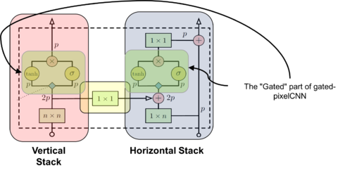
In essence, PixelCNN typically consists of a stack of masked convolutional layers that takes an $N \times N \times 3$ image as input and produces $N \times N \times 3 \times 256$ (probability of pixel intensity) predictions as output. During sampling the predictions are sequential: every time a pixel is predicted, it is fed back into the network to predict the next pixel. This sequentiality is essential to generating high quality images, as it allows every pixel to depend in a highly non-linear and multimodal way on the previous pixels.
Another important mention is that the residual connections are only for horizontal stacks. On the other side skip connections allow as to incorporate features from all layers at the very end of out network. Most important stuff to mention here is that skip and residual connection use different weights after gated block.
Conditional PixelCNN
Conditioning is a smart word for saying that we’re feeding the network some high-level information - for instance, providing an image to the network with the associated classes in MNIST/CIFAR datasets. During training you feed image as well as class to your network to make sure network would learn to incorporate that information as well. During inference you can specify what class your output image should belong to. You can pass any information you want with conditioning, we’ll start with just classes.
For a conditional PixelCNN, we represent a provided high-level image description as a latent vector $h$, wherein the purpose of the latent vector is to model the conditional distribution $p(x|h)$ such that we get a probability as to if the images suites this description. The conditional PixelCNN models based on the following distribution:
$$p(x|h) = \prod\limits_{i=1}^{n^2} p(x_i | x_1, ..., x_{i-1}, h)$$
Hence, now the conditional distribution is dependent on the latent vector h, which is now appended onto the activations prior to the non-linearities; hence the activation function after adding the latent vector becomes:
$$y = tanh(W_{k,f} \ast x + V_{k,f}^T h) \odot \sigma(W_{k,g} \ast x + V_{k,g}^T h)$$
Note $h$ multiplied by matrix inside tanh and sigmoid functions, $V$ matrix has the shape [number of classes, number of filters], $k$ is the layer number, and the classes were passed as a one-hot vector $h$ during training and inference.
Note that if the latent vector h is a one-hot encoding vector that provides the class labels, which is equivalent to the adding a class dependent bias at every layer. So, this means that the conditioning is independent of the location of the pixel - this is only if the latent vector holds information about “what should the image contain” rather than the location of contents in the image. For instance, we could specify that a certain animal or object should appear in different positions, poses, and backgrounds.
Note that this conditioning does not depend on the location of the pixel in the image. To consider the location as well, this is achieved by mapping the latent vector $h$ to a spatial representation $s=m(h)$ (which contains the same dimension of the image but may have an arbitrary number of feature maps) with a deconvolutional neural network $m()$; this provides a location dependent bias as follows:
$$y = tanh(W_{k,f} \ast x + V_{k,f} \ast s) \odot \sigma(W_{k,g} \ast x + V_{k,g} \ast s)$$
where $V_{k,g}\ast s$ is an unmasked $1\times1$ convolution.
PixelCNN Auto-Encoders
Since conditional PixelCNNs can model images based on the distribution $p(x|h)$, it is possible to apply this analogy into image decoders used in auto-encoders. Introduced by Hinton et. al in [5], autoencoder is a dimensionality reduction neural network which is composed of two parts: an encoder which maps the input image into low-dimensional representation (i.e. the latent vector $h$) , and a decoder that decompresses the latent vector to reconstruct the original image.
In order to apply the conditional PixelCNN onto the autoencoder, the deconvolutional decoders are replaced with the conditional PixelCNN - the re-architectured network of which is used for training a data set. It starts with a traditional convolutional auto-encoder architecture as in [12]. The deconvolutional decoder is replaced with PixelCNN and the network is trained end-to-end. The authors observe that the encoder can better extract representations of the provided input data - this is because much of the low-level pixel statistics is now handled by the PixelCNN; hence, the encoder omits low-level pixel statistics and focuses on more high-level abstract information. Since the release of the present work, other authors have started using PixelCNN for/as part of their auto-encoders. In particular, a recent work used PixelCNN within a generative adversarial network [13].
Experiments
Unconditional Modelling with Gated PixelCNN
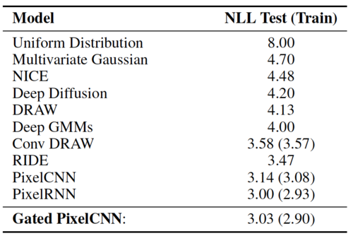
For the first set of experiments, the authors evaluate the Gated PixelCNN unconditioned model on the CIFAR-10 dataset is adopted. A comparison of the validation score between the Gated PixelCNN, PixelCNN, and PixelRNN is computed, wherein the lower score means that the optimized model generalizes better. Using the negative log-likelihood criterion (NLL), the Gated PixelCNN obtains an NLL Test (Train) score of 3.03 (2.90) which outperforms the PixelCNN by 0.11 bits/dim, which obtains 3.14 (3.08). Although the performance is a bit better, visually the quality of the samples that were produced is much better for the Gated PixelCNN when compared to PixelCNN. It is important to note that the Gated PixelCNN came close to the performance of PixelRNN, which achieves a score of 3.00 (2.93). Table 1 provides the test performance of benchmark models on CIFAR-10 in bits/dim (where lower is better), and the corresponding training performance is in brackets.
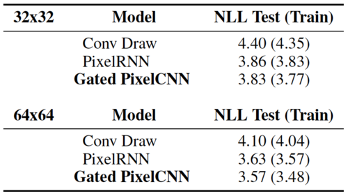
Another experiment on the ImageNet data is performed for image sizes $32 \times 32$ and $64 \times 64$. In particular, for a $32 \times 32$ image, the Gated PixelCNN obtains a NLL Test (Train) of 3.83 (3.77) which outperforms PixelRNN which achieves 3.86 (3.83); from which the authors observe that larger models do have better performance, however, the simpler PixelCNN does have the ability to scale better. For a $64 \times 64$ image, the Gated PixelCNN obtains 3.57 (3.48) which, yet again, outperforms PixelRNN which achieves 3.63 (3.57). The authors do mention that the Gated PixelCNN performs similarly to the PixelRNN (with row LSTM); however, Gated PixelCNN is observed to train twice as quickly at 60 hours when using 32 GPUs. The Gated PixelCNN has 20 layers (Figure 2), each of which has 384 hidden units and a filter size of 5x5. For training, a total of 200K synchronous updates were made over 32 GPUs which were computed in TensorFlow using a total batch size of 128. Table 2 illustrates the performance of benchmark models on ImageNet dataset in bits/dim (where lower is better) and the training performance in brackets.
Conditioning on ImageNet Classes
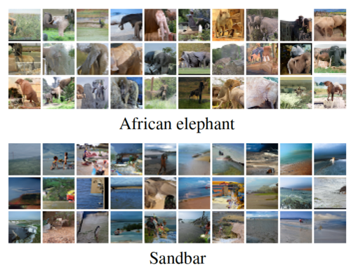
For the second set of experiments, the authors evaluated the Gated PixelCNN model by conditioning the classes of the ImageNet images. Using the one-hot encoding $(h_i)$, for which the $i^th$ class the distribution becomes $p(x|h_i)$, the model receives roughly log(1000) $\approx$ 0.003 bits/pixel for a $32 \times 32$ image. Although the log-likelihood did not show a significant improvement, visually the quality of the images were generated much better when compared to the original PixelCNN.
Figure 11 shows some samples from 8 different classes of ImageNet images from a single class-conditioned model. It is evident that the Gated PixelCNN can better distinguish between objects, animals and backgrounds. The authors observe that the model can generalize and generate new renderings from the animal and object class when the trained model is provided with approximately 1000 images.
Conditioning on Portrait Embeddings
For the third set of experiments, the authors used the top layer of the CNN trained on a large database of portraits that were automatically cropped from Flickr images using face detector. This pre-trained network was trained using triplet loss function which ensured a similar the latent embeddings for particular face across the entire dataset. The motivation of the triplet loss function (Schroff et al.) is to ensure that an image $x^a_i$ (anchor) of a specific person is close to all other images $x^p_i$ (positive) of the same person than it is to any image $x^n_i$ (negative) of any other person. So the tuple loss function is given by \[ L = \sum_{i} [||h(x^a_i)-h(x^p_i)) ||^2_2- ||h(x^\alpha_i)-h(x^n_i)) ||^2_2 +\alpha ]_+ \] where $h$ is the embedding of the image $x$, and $\alpha$ is a margin that is enforced between positive and negative pairs.
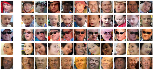
In essence, the authors took the latent vector from this supervised pre-trained network which now has the architecture (image=$x$, embedding=$h$) tuples and trained the Conditional PixelCNN with the latent embeddings to model the distribution $p(x|h)$. Hence, if the network is provided with a face that is not in the training set, the model now has the capability to compute the latent embeddings $h=f(x)$ such that the output will generate new portraits of the same person. Figure 12 provides a pictorial example of the aforementioned manipulated network where it is evident that the generative model can produce a variety of images, independent from pose and lighting conditions, by extracting the latent embeddings from the pre-trained network.
PixelCNN Auto Encoder
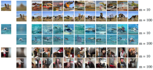
For the final set of experiment, the authors venture the possibility to train the Gated PixelCNN by adopting the Autoencoder architecture. The authors start by training a PixelCNN auto-encoder using $32 \times 32$ ImageNet patches and compared its results to a convolutional autoencoder, optimized using mean-square error. It is important to note that both the models use a 10 or 100 dimensional bottleneck.
Figure 13 provides a reconstruction using both the models. It is evident that the latent embedding produced when using PixelCNN autoencoder is much different when compared to convolutional autoencoder. For instance, in the last row, the PixelCNN autoencoder is able to generate similar looking indoor scenes with people without directly trying to "reconstruct" the input, as done by the convolutional autoencoder.
Conclusion
This work introduced the Gated PixelCNN which is an improvement over the original PixelCNN. In addition to the Gated PixelCNN being more computationally efficient, it now has the ability to match, and in some cases, outperform PixelRNN. In order to deal with the "blind spots" in the receptive fields presented in the PixelCNN, the newly proposed Gated PixelCNN use two CNN stacks (horizontal and vertical filters) to deal with this problem. Moreover, the authors now use a custom-made tank and sigmoid function over the ReLU activation functions because these multiplicative units helps to model more complex interactions. The proposed network obtains a similar performance to PixelRNN on CIFAR-10, however, it is now state-of-the-art on the ImageNet $32 \times 32$ and $64 \times 64$ datasets.
In addition, the conditional PixelCNN is also explored on natural images using three different settings. When using class-conditional generation, the network showed that a single model is able to generate diverse and realistic looking images corresponding to different classes. When looking at generating human portraits, the model does have the ability to generate new images from the same person in different poses and lighting conditions given a single image. Finally, the authors also showed that the PixelCNN can be used as image decoder in an autoencoder. Although the log-likelihood is quite similar when comparing it to literature, the samples generated from the PixelCNN autoencoder model does provide high visual quality images showing natural variations of objects and lighting conditions.
Summary
$\bullet$ Improved PixelCNN called Gated PixelCNN
- Similar performance as PixelRNN, and quick to compute like PixelCNN (since it is easier to parallelize)
- Fixed the "blind spot" problem by introducing 2 stacks (horizontal and vertical)
- Gated activation units which now use sigmoid and tanh instead of ReLU units
$\bullet$ Conditioned Image Generation
- One-shot conditioned on class-label
- Conditioned on portrait embedding
- PixelCNN AutoEncoders
$\bullet$ Future Works
- Combining Conditional PixelCNNs with variational inference to create a variational auto-encoder.
- Modeling images based on an image caption instead of the class label.
Critique
- The paper is not descriptive and does not explain well on how the horizontal and vertical stacks solve the "blindspot" problem. In addition, the authors just mention the "gated block" and how they designed it, but they do not explain the intuition and how this approach is an improvement over the PixelCNN
- The authors do not provide a good pictorial representation on any of the aforementioned novelties
- The PixelCNN AutoEncoder is not descriptive enough!
- It seems that the model is giving very clear quality images due to a combination of newly introduced components such as two-stack architecture, residual-connection and gating nonlinearities. But the paper doesn't say which of these tricks had the highest impact. An experimental study on the same would have been informative.
- Also the description or source of the dataset "portraits" is not provided that help assess experimental result quality.
- The reasons for the introduction of gating nonlinearities, the two-stack architecture, and the residual connections in the horizontal stack are not detailed discussed in this paper.
- A quantitative comparison of the novel model with VAEs and GANs is not given.
- An alternative method of tackling the "blind spot" problem would be to increase the effective receptive field size itself [10]. This can be done in two ways:
- Increasing the depth of the convolution filters
- Adding subsampling layers
- It is not made explicit how the author's handle image boundaries
- The architecture cannot be (easily) parallelized, making alternative methods far more efficient computationally (a concern that matter deeply in practice)
Followup
Variational Autoencoders (VAEs) learn a useful latent representation and model global structure well but have difficulty capturing small details. PixelCNN (this paper) models details very well, but lacks a latent code and is difficult to scale for capturing large structures. PixelVAE, a VAE model with an autoregressive decoder based on PixelCNN was introduced as a followup on this, which requires very few expensive autoregressive layers compared to PixelCNN and learns latent codes that are more compressed than a standard VAE while still capturing most non-trivial structure.
Reference
- Aaron van den Oord et al., "Pixel Recurrent Neural Network", ICML 2016
- Aaron van den Oord et al., "Conditional Image Generation with PixelCNN Decoders", NIPS 2016
- S. Turukin, "Gated PixelCNN", Sergeiturukin.com, 2017. [Online]. Available: http://sergeiturukin.com/2017/02/24/gated-pixelcnn.html. [Accessed: 15- Nov- 2017].
- S. Reed, A. van den Oord, N. Kalchbrenner, V. Bapst, M. Botvinick and N. Freitas, "Generating interpretable images with controllable structure", 2016.
- G. Hinton, "Reducing the Dimensionality of Data with Neural Networks", Science, vol. 313, no. 5786, pp. 504-507, 2006.
- "Conditional Image Generation with PixelCNN Decoders", Slideshare.net, 2017. [Online]. Available: https://www.slideshare.net/suga93/conditional-image-generation-with-pixelcnn-decoders. [Accessed: 18- Nov- 2017].
- "Gated PixelCNN", Kawahara.ca, 2017. [Online]. Available: http://kawahara.ca/conditional-image-generation-with-pixelcnn-decoders-slides/gated-pixelcnn/. [Accessed: 17- Nov- 2017].
- K. Dhandhania, "PixelCNN + PixelRNN + PixelCNN 2.0 — Commonlounge", Commonlounge.com, 2017. [Online]. Available: https://www.commonlounge.com/discussion/99e291af08e2427b9d961d41bb12c83b. [Accessed: 15- Nov- 2017].
- S. Turukin, "PixelCNN", Sergeiturukin.com, 2017. [Online]. Available: http://sergeiturukin.com/2017/02/22/pixelcnn.html. [Accessed: 17- Nov- 2017].
- W. Luo, Y. Li, R. Urtasun, and R. Zemel. Understanding the effective receptive field in deep convolutional neural networks. arXiv preprint arXiv:1701.04128, 2017
- https://www.commonlounge.com/discussion/312f295cf49f4905b1a41897a64efc98
- Masci J., Meier U., Cireşan D., Schmidhuber J. (2011) Stacked Convolutional Auto-Encoders for Hierarchical Feature Extraction. In: Honkela T., Duch W., Girolami M., Kaski S. (eds) Artificial Neural Networks and Machine Learning – ICANN 2011. ICANN 2011. Lecture Notes in Computer Science, vol 6791. Springer, Berlin, Heidelberg
- A. Makhzani, B. Frey. PixelGAN Autoencoders. arXiv preprint (2017).
Implement reference: https://github.com/anantzoid/Conditional-PixelCNN-decoder