contributions on Quantifying Cancer Progression with Conjunctive Bayesian Networks

Motivation

Tumor progression is characterized by a sequence of multiple genetic mutations that arise due to activation of oncogenes and inactivation of tumor suppressor genes. It is still unknown about the temporal order of these mutations, as carcinogenic process is a slow process and takes several years. Biologically motivated mathematical models such as "Evolutionary dynamics" have been used to describe the sequence of events. Several statistical models such as oncogenetic trees, network trees, probabilistic network models, etc have been used to model disease progression, in particular cancer. Genetic events happen in no specific order, due to which a single node can have multiple parents. This lead to the use of a more generalization framework for tree models called as the conjunctive Bayesian networks. In simple words, a conjunctive Bayesian network is a directed acyclic graph that allows for multiple parent nodes. One biggest advantage of this model is that it can model multiple mutational pathways.

Introduction

A poset [math]\displaystyle{ P }[/math] or a partially ordered set has a binary relation "[math]\displaystyle{ \lt }[/math]" which has the following properties:

• Reflexive
• Antisymmetry
• Transitive

In this model, [math]\displaystyle{ P }[/math] denotes the set of mutational events and the binary relation defines the order of occurrence of the constraints. For example, [math]\displaystyle{ p \lt q }[/math] denotes that mutation [math]\displaystyle{ q }[/math] can occur only after the occurrence of mutation [math]\displaystyle{ p }[/math]. We denote [math]\displaystyle{ p }[/math] as the parent of [math]\displaystyle{ q }[/math] if there exists no node [math]\displaystyle{ r \in P }[/math] such that [math]\displaystyle{ r\neq p }[/math], [math]\displaystyle{ r\neq q }[/math] and [math]\displaystyle{ p\lt r\lt q }[/math]. Denote [math]\displaystyle{ p\rightarrow q }[/math] to say that [math]\displaystyle{ p }[/math] is the parent of [math]\displaystyle{ q }[/math]. The set of all parents is denoted by [math]\displaystyle{ pa(q) }[/math]. We now construct the distributive lattice of order ideals of [math]\displaystyle{ P }[/math] denoted by [math]\displaystyle{ J(P) }[/math]. The distributive lattice is defined as follows: all the subsets [math]\displaystyle{ S\subset P }[/math] and [math]\displaystyle{ S\in J(P) }[/math]. We say that [math]\displaystyle{ S\in J(P) }[/math] if and only if for all [math]\displaystyle{ q\in S }[/math] and [math]\displaystyle{ p \lt q }[/math] then [math]\displaystyle{ p\in S }[/math].

A conjunctive Bayesian network (CBN) is characterized by a set of events [math]\displaystyle{ E }[/math] along with a partial order "[math]\displaystyle{ \lt }[/math]" that is defined on the events and with parameters [math]\displaystyle{ \theta_e }[/math] for each events [math]\displaystyle{ e\in E }[/math]. The state space of this CBN is the distributive lattice [math]\displaystyle{ J(E) }[/math] of order ideals in the events set [math]\displaystyle{ E }[/math]. Elements of distributive lattice are called as genotypes. To summarize, a CBN is:

• a model that places partial order on the genetic mutations
• assumes total number of mutations as fixed, say [math]\displaystyle{ n }[/math]
• model assumes no reverse mutations at any point of time in the process
• generates a lattice of possible genotypes

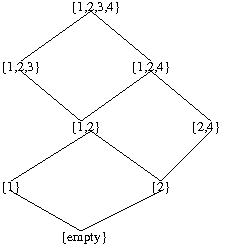
Here is a simple example that illustrates a poset and construction of distributive lattice taken from <ref name="R1"> Beerenwinkel N. and Sullivant S, “Markov models for accumulating mutations,” in Biometrika, 96, 3 ,pp. 645–661, 2009.</ref>

A poset that is defined on the four element set as [math]\displaystyle{ [4]={1,2,3,4} }[/math] constrained on the binary relation [math]\displaystyle{ 1\lt 3 }[/math], [math]\displaystyle{ 2\lt 3 }[/math] and [math]\displaystyle{ 2\lt 4 }[/math].

Fig.1 A sample poset with 4 mutations

We notice that mutation 3 cannot happen until the occurrence of mutations 1 and 2. Mutation 4 cannot happen until the occurrence of mutation 2. Then the distributive lattice can be constructed as follows for Fig 1:

Fig.2 lattice of order ideals

Bayesian networks and detection of cancer

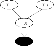
A tumor has to grow to a minimum size in order to detect it using CT scans or MRI scans. Firstly, a malignant tumor has to grow to a particular size and secondly the clinical diagnosis has to be correct. A model is formulated as follows:

• [math]\displaystyle{ T }[/math]: Waiting time for tumor to develop
• [math]\displaystyle{ T_s }[/math]: Waiting time for clinical diagnosis

The dynamics of CBN is a hidden process due to one of the observation variable, and hence this model is treated as a hidden CBN. Figure 3 shows a simple CBN with a hidden process.

Fig.3 Sample CBN for cancer diagnosis

Both the times defined above are random variables. In general, [math]\displaystyle{ T }[/math] and [math]\displaystyle{ T_s }[/math] are not known due to which we assume that both are independent. Therefore their joint distribution is given by [math]\displaystyle{ f(t,t_s)=f(t)f(t_s) }[/math]. Cancer is detected only when it is observed during the diagnosis time. Suppose [math]\displaystyle{ X\in{0,1} }[/math] be a binary random variable that indicates presence of cancer at [math]\displaystyle{ T_s }[/math]. If cancer is diagnosed at [math]\displaystyle{ T_s }[/math] then [math]\displaystyle{ X }[/math] is set to be one. Then the probability of [math]\displaystyle{ X }[/math] is given by:

[math]\displaystyle{ Prob(X) = \int_0^{\infty}\int_0^{\infty}Prob(X|T=t,T_s=t_s)f(t)f(t_s)dt dt_s }[/math]

where the conditional probability

[math]\displaystyle{ Prob(X=1|T=t,T_s=t_s)=I(t\lt t_s) }[/math]

is called as the indicator function. Model described above assumes that diagnosis is always correct. Practically, there is always a chance that diagnosis might go wrong. Let us suppose that diagnosis is overlooked or misdiagnosed with a probability [math]\displaystyle{ \epsilon }[/math]. This assumption leads us to saying that, clinical diagnosis is also regarded a probabilistic event [math]\displaystyle{ Y }[/math] that depends on [math]\displaystyle{ X }[/math]. Hence, the probability of [math]\displaystyle{ Y }[/math] is given by

[math]\displaystyle{ Prob(Y) = \sum _{X=0,1}Prob_{\epsilon}(Y|X)Prob(X) }[/math]

where [math]\displaystyle{ Prob(X) }[/math] is defined as above and,

[math]\displaystyle{ Prob_{\epsilon}(Y|X)= \epsilon^{I(Y\neq X)} (1-\epsilon)^{I(Y=X)} }[/math]

Variables [math]\displaystyle{ {T,T_s,X,Y} }[/math] form a Bayesian network and the joint density can be factorized into conditional densities.

Notes

Beerenwinkel (one of the authors) previously put some assumptions and followed them when modelling the accumulative evolutionary process. Such assumptions are:

1. Substitutions do not occur independently. There are preferred evolutionary pathways in which mutations are fixed

2. The fixation mutations into the population is definite. This means that substitutions are non-reversible

3. At each time point, the virus population is dominated by a single strain and clones are independent and (sometimes erroneous) copies of this genotype

Improvements

As mentioned in the paper, an improvement on the proposed model would be to use different parameters [math]\displaystyle{ \varepsilon^+ }[/math] and [math]\displaystyle{ \varepsilon^- }[/math] for false positives and false negatives in the error model. Beerenwinkel and Drton have developed this idea.

Let [math]\displaystyle{ \varepsilon^+ = (\varepsilon_1^+,...,\varepsilon_M^+) \in [0, 1]^M }[/math] and [math]\displaystyle{ \varepsilon^- = (\varepsilon_1^-,...,\varepsilon_M^-) \in [0, 1]^M }[/math] be parameter vectors that contain the mutation specific probabilities of observing a false positive and a false negative respectively. False positives (negatives) are mutations observed in clones derived from a virus population that is in mutant state at such time point. The false positive and false negative negative rates summarize differences from the population state. Then, these parameters quantify the expected genetic diversity of the virus population. Conditionally upon the hidden state [math]\displaystyle{ X_{jm} }[/math], the probabilities of observing mutation [math]\displaystyle{ m }[/math] in clone [math]\displaystyle{ k }[/math] at time point [math]\displaystyle{ t_j }[/math] are as follows:

[math]\displaystyle{ \begin{matrix} \theta^l(\varepsilon_m^+, \varepsilon_m^-) = \begin{matrix} & 0 & 1\\ 0 & 1-\varepsilon_m^+ & \varepsilon_m^+\\ 1 & \varepsilon_m^- & 1-\varepsilon_m^- \end{matrix} \end{matrix} }[/math]

The entries of this matrix are the conditional probabilities

[math]\displaystyle{ \begin{matrix} \theta^l(\varepsilon_m^+, \varepsilon_m^-)_{x_{jm},y_{jkm}} = Prob(Y_{jkm}=y_{jkm}|X_{jm}=x_{jm}) \end{matrix} }[/math]

then the model is concluded accordingly.

References

<references />