Self-Supervised Learning of Pretext-Invariant Representations
Presented by
Sina Farsangi
Introduction
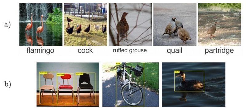
Modern image recognition and object detection systems find image representations using a large number data with pre-defined semantic annotation. Some examples of these annotations are class labels and bonding boxes as shown in Figure 1. For finding representations using pre-defined semantic annotations, there is a need for large number of labeled data which is not the case in all scenarios. Also, these systems usually learn features that are specific for a particular type of class and not necessarily semantically meaningful features that can help to generalize to other domains and classes. In other words, pre-defined semantic annotations scale poorly to the long scale of visual concepts[1]. Therefore, there has been a big interest in the community to find image representations that are more visually meaningful and can help in several tasks such as image recognition and object detection. One of the fast growing areas of research that tries to address this problem is Self-Supervised Learning. Self-Supervised Learning tries to learn deep models that find image representations from the pixels themselves rather than using pre-defined semantic annotated data. As we will show, there is no need for using class labels [1] or bounding boxes [2] in self-supervised learning.
Self-Supervised Learning is often done using a set of tasks called Pretext tasks. During these tasks, a transformation [math]\displaystyle{ \tau }[/math] is applied to unlabeled images [math]\displaystyle{ I }[/math] to obtain a set of transformed images, [math]\displaystyle{ I^{t} }[/math]. Then, a deep neural network, [math]\displaystyle{ \phi(\theta) }[/math], is trained to predict the transformation characteristic. Several Pretext Tasks exist based on the type of used transformation. Two of the most used pretext tasks are rotations and jigsaw puzzle [3,4,5]. As shown in Figure 2, in the rotation task, unlabeled images, [math]\displaystyle{ }[/math] are rotated by random degrees (0,90,180,270) and the deep network learns to predict the rotation degree. Also, in jigsaw task which is more complicated than rotation task, unlabeled images are cropped into 9 patches and then, the image is perturbed by randomly permuting the nine patches. Then, a deep network is trained to predict the permutation of the patches in the perturbed image.

Although the proposed pretext tasks have obtained promising results, they have the disadvantage of being covariant to the applied transformation. In other words, as deep networks are trained to predict transformations characteristics, they will also learn representations that will vary based on the applied transformation. By intuition, we would like to obtain representations the are common between the original images and the transformed ones. This idea is supported by the fact that humans are able to recognize these transformed images. This hints us to try to develop a method that obtains image representations that are common between the original and transformed images, in other words, image representations that are transformation invariant. The summarized paper tries to address this problem by introducing Pretext Invariant Representation Learning (PIRL) that learns to obtain self-supervised image representations that as opposed to Pretext tasks are transformation invariant and therefore, more semantically meaningful. The performance of the proposed method is evaluated on several self-supervision learning benchmarks. The results show that the PIRL introduces a new state-of-the-art method in Self-Supervised Learning by learning transformation invariant representations.
Methodology
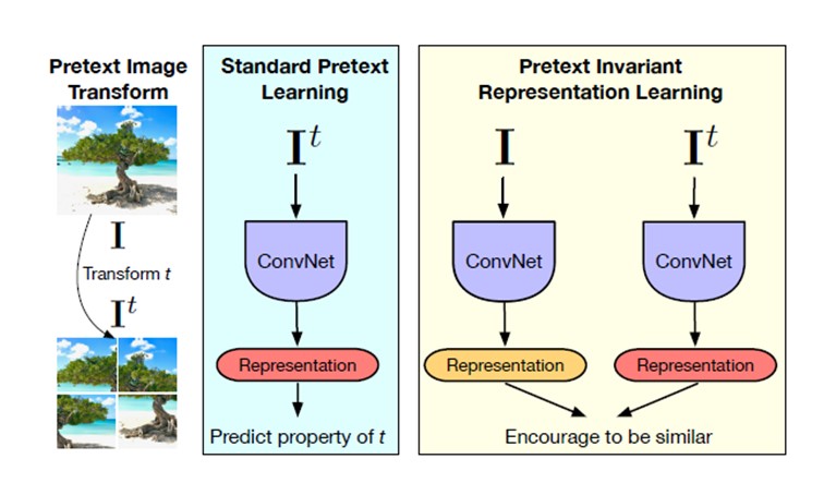
An overview of the proposed method and a comparison with Pretext Tasks are shown in Figure 3. For a given image in the Dataset of unlabeled images [math]\displaystyle{ D=\{{I_1,I_2,...,I_{|D|}}\} }[/math], [math]\displaystyle{ I }[/math], a transformation [math]\displaystyle{ \tau }[/math] is applied:
\begin{align} \tag{1} \label{eqn:1} I^t=\tau(I) \end{align} where [math]\displaystyle{ I^t }[/math] is the transformed image. We would like to train a convolutional neural network, [math]\displaystyle{ \phi(\theta) }[/math] that constructs image representations [math]\displaystyle{ v_{I}=\phi_{\theta}(I) }[/math]. Pretext Task based methods learn to predict transformation characteristics, [math]\displaystyle{ z(t) }[/math], by minimizing a transformation covariant loss function in the form of:
\begin{align} \tag{2} \label{eqn:1} l_{\text{cov}}(\theta,D)=\frac{1}{|D|} \sum_{I \in {D}}^{} L(v_I,z(t) \end{align}
One of the major parameters that can be changed in the JPEG pipeline is the quantization table, which is the main source of artifacts added in the image to make it lossless compression as shown in [1, 4]. The authors got motivated to change the JPEG configuration to optimize the uploading rate of different cloud computer vision without considering pre-knowledge of the original model and dataset. In contrast to the authors in [2, 3, 5] where they adjust the JPEG configuration by retraining the parameters or according to the structure of the model. They considered the lack of undefined quantization level which decreases the image rate and quality but the deep learning model can still recognize it as shown in [4]. The authors in [1] used Deep Reinforcement learning (DRL) in an online manner to choose the quantization level to upload an image to the cloud for the computer vision model and this is the only approach to design an adaptive JPEG based on RL mechanism.
The approach is designed based on an interactive training environment which represents any computer vision cloud services, then they needed a tool to evaluate and predict the performance of quantization level on an uploaded image, so they used a deep Q neural network agent. They feed the agent with a reward function which considers two optimization parameters, accuracy and image size. It works as iterative behavior interacting with the environment. The environment is exposed to different images with different virtual redundant information that needs an adaptive solution for each image to select the suitable compression level for the model. Thus, they designed an explore-exploit mechanism to train the agent on different scenery which is designed in deep Q agent as an inference-estimate-retain mechanism to restart the training procedure for each image. The authors verify their approach by providing some analysis and insight using Grad-Cam [8] by showing some patterns of how a compression level is chosen for each image with its own corresponding quality factor. Each image shows a different response when shown to a deep learning model. In general, images are more sensitive to compression if they have large smooth areas, while those with complex textures are more robust to compression.
What is a quantization table?
Before getting to the quantization table first look at the basic architecture of JPEG's baseline system. This has 4 blocks, which are FDCT (Fast Discrete Cosine Transformation), quantizer, statistical model, and entropy encoder. The FCDT block takes an input image separated into [math]\displaystyle{ n \times n }[/math] blocks and applies a discrete cosine transformation creating DCT terms. These DCT terms are values from a relatively large discrete set that will be then mapped through the process of quantization to a smaller discrete set. This is accomplished with a quantization table at the quantizer block, which is designed to preserve low-frequency information at the cost of the high-frequency information. This preference for low frequency information is made because losing high frequency information isn't as impactful to the image when perceived by a humans visual system.
Problem Formulation
The authors formulate the problem by referring to the cloud deep learning service as [math]\displaystyle{ \vec{y}_i = M(x_i) }[/math] to predict results list [math]\displaystyle{ \vec{y}_i }[/math] for an input image [math]\displaystyle{ x_i }[/math], and for reference input [math]\displaystyle{ x \in X_{\rm ref} }[/math] the output is [math]\displaystyle{ \vec{y}_{\rm ref} = M(x_{\rm ref}) }[/math]. It is referred [math]\displaystyle{ \vec{y}_{\rm ref} }[/math] as the ground truth label and also [math]\displaystyle{ \vec{y}_c = M(x_c) }[/math] for compressed image [math]\displaystyle{ x_{c} }[/math] with quality factor [math]\displaystyle{ c }[/math].
\begin{align} \tag{1} \label{eq:accuracy}
\mathcal{A} =& \sum_{k}\min_jd(l_j, g_k) \\
& l_j \in \vec{y}_c, \quad j=1,...,5 \nonumber \\
& g_k \in \vec{y}_{\rm ref}, \quad k=1, ..., {\rm length}(\vec{y}_{\rm ref}) \nonumber \\
& d(x, y) = 1 \ \text{if} \ x=y \ \text{else} \ 0 \nonumber
\end{align}
The authors divided the used datasets according to their contextual group [math]\displaystyle{ X }[/math] according to [6] and they compare their results using compression ratio [math]\displaystyle{ \Delta s = \frac{s_c}{s_{\rm ref}} }[/math], where [math]\displaystyle{ s_{c} }[/math] is the compressed size and [math]\displaystyle{ s_{\rm ref} }[/math] is the original size, and accuracy metric [math]\displaystyle{ \mathcal{A}_c }[/math] which is calculated based on the hamming distance of Top-5 of the output of softmax probabilities for both original and compressed images as shown in Eq. \eqref{eq:accuracy}. In the RL designing stage, continuous numerical vectors are represented as the input features to the DRL agent which is Deep Q Network (DQN). The challenges of using this approach are: (1) The state space of RL is too large to cover, so the neural network is typically constructed with more layers and nodes, which makes the DRL agent hard to converge and the training time-consuming; (2) The DRL always starts with a random initial state, but it needs to find a higher reward before starting the training of the DQN. However, the sparse reward feedback resulted from a random initialization makes learning difficult. The authors solve this problem by using a pre-trained small model called MobileNetV2 as a feature extractor [math]\displaystyle{ \mathcal{E} }[/math] for its ability in lightweight and image classification, and it is fixed during training the Q Network [math]\displaystyle{ \phi }[/math]. The last convolution layer of [math]\displaystyle{ \mathcal{E} }[/math] is connected as an input to the Q Network [math]\displaystyle{ \phi }[/math], so by optimizing the parameters of Q network [math]\displaystyle{ \phi }[/math], the RL agent's policy is updated.
Reinforcement learning framework
This paper [1] described the reinforcement learning problem as [math]\displaystyle{ \{\mathcal{X}, M\} }[/math] to be emulator environment, where [math]\displaystyle{ \mathcal{X} }[/math] is defining the contextual information created as an input from the user [math]\displaystyle{ x }[/math] and [math]\displaystyle{ M }[/math] is the backend cloud model. Each RL frame must be defined by action and state, the action is known by 10 discrete quality levels ranging from 5 to 95 by step size of 10 and the state is feature extractor's output [math]\displaystyle{ \mathcal{E}(J(\mathcal{X}, c)) }[/math], where [math]\displaystyle{ J(\cdot) }[/math] is the JPEG output at specific quantization level [math]\displaystyle{ c }[/math]. They found the optimal quantization level at time [math]\displaystyle{ t }[/math] is [math]\displaystyle{ c_t = {\rm argmax}_cQ(\phi(\mathcal{E}(f_t)), c; \theta) }[/math], where [math]\displaystyle{ Q(\phi(\mathcal{E}(f_t)), c; \theta) }[/math] is action-value function, [math]\displaystyle{ \theta }[/math] indicates the parameters of Q network [math]\displaystyle{ \phi }[/math]. In the training stage of RL, the goal is to minimize a loss function [math]\displaystyle{ L_i(\theta_i) = \mathbb{E}_{s, c \sim \rho (\cdot)}\Big[\big(y_i - Q(s, c; \theta_i)\big)^2 \Big] }[/math] that changes at each iteration [math]\displaystyle{ i }[/math] where [math]\displaystyle{ s = \mathcal{E}(f_t) }[/math] and [math]\displaystyle{ f_t }[/math] is the output of the JPEG, and [math]\displaystyle{ y_i = \mathbb{E}_{s' \sim \{\mathcal{X}, M\}} \big[ r + \gamma \max_{c'} Q(s', c'; \theta_{i-1}) \mid s, c \big] }[/math] is the target that has a probability distribution [math]\displaystyle{ \rho(s, c) }[/math] over sequences [math]\displaystyle{ s }[/math] and quality level [math]\displaystyle{ c }[/math] at iteration [math]\displaystyle{ i }[/math], and [math]\displaystyle{ r }[/math] is the feedback reward.
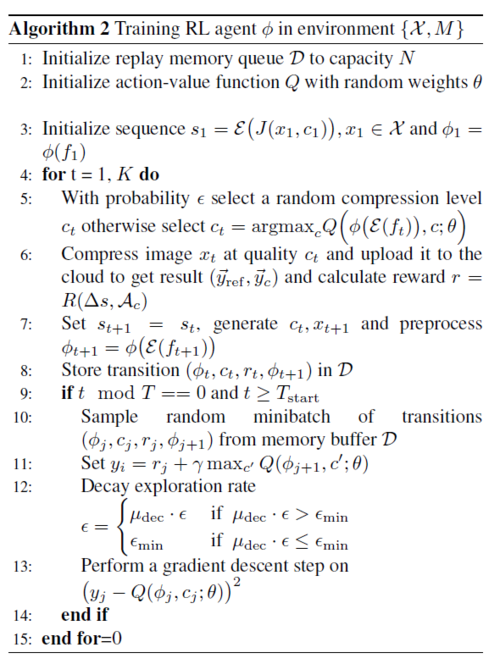
The framework get more accurate estimation from a selected action when the distance of the target and the action-value function's output [math]\displaystyle{ Q(\cdot) }[/math] is minimized. As a results, no feedback signal can tell that an episode has finished a condition value [math]\displaystyle{ T }[/math] that satisfies [math]\displaystyle{ t \geq T_{\rm start} }[/math] to guarantee to store enough transitions in the memory buffer [math]\displaystyle{ D }[/math] to train on. To create this transitions for the RL agent, random trials are collected to observe environment reaction. After fetching some trials from the environment with their corresponding rewards, this randomness is decreased as the agent is trained to minimize the loss function [math]\displaystyle{ L }[/math] as shown in the Algorithm below. Thus, it optimizes its actions on a minibatch from [math]\displaystyle{ \mathcal{D} }[/math] to be based on historical optimal experience to train the compression level predictor [math]\displaystyle{ \phi }[/math]. When this trained predictor [math]\displaystyle{ \phi }[/math] is deployed, the RL agent will drive the compression engine with the adaptive quality factor [math]\displaystyle{ c }[/math] corresponding to the input image [math]\displaystyle{ x_{i} }[/math].
The interaction between the agent and environment [math]\displaystyle{ \{\mathcal{X}, M\} }[/math] is evaluated using the reward function, which is formulated, by selecting an appropriate action of quality factor [math]\displaystyle{ c }[/math], to be directly proportional to the accuracy metric [math]\displaystyle{ \mathcal{A}_c }[/math], and inversely proportional to the compression rate [math]\displaystyle{ \Delta s = \frac{s_c}{s_{\rm ref}} }[/math]. As a result, the reward function is given by [math]\displaystyle{ R(\Delta s, \mathcal{A}) = \alpha \mathcal{A} - \Delta s + \beta }[/math], where [math]\displaystyle{ \alpha }[/math] and [math]\displaystyle{ \beta }[/math] to form a linear combination.
Inference-Estimate-Retrain Mechanism
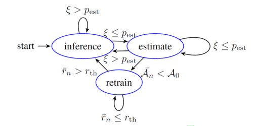
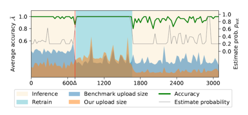
The system diagram, AdaCompress, is shown in figure 3 in contrast to the existing modules. When the AdaCompress is deployed, the input images scenery context [math]\displaystyle{ \mathcal{X} }[/math] may change, in this case the RL agent’s compression selection strategy may cause the overall accuracy to decrease. So, in order to solve this issue, the estimator will be invoked with probability [math]\displaystyle{ p_{\rm est} }[/math]. This will be done by generating a random value [math]\displaystyle{ \xi \in (0,1) }[/math] and the estimator will be invoked if [math]\displaystyle{ \xi \leq p_{\rm est} }[/math]. Then AdaCompress will upload both the original image and the compressed image to fetch their labels. The accuracy will then be calculated and the transition, which also includes the accuracy in this step, will be stored in the memory buffer. Comparing recent the n steps' average accuracy with earliest average accuracy, the estimator will then invoke the RL training kernel to retrain if the recent average accuracy is much lower than the initial average accuracy.
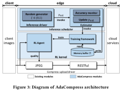
The authors solved the change in the scenery at the inference phase that might cause learning to diverge by introducing running-estimate-retain mechanism. They introduced estimator with probability [math]\displaystyle{ p_{\rm est} }[/math] that changes in an adaptive way and it is compared a generated random value [math]\displaystyle{ \xi \in (0,1) }[/math]. As shown in Figure 2, Adacompression is switching between three states in an adaptive way as will be shown in the following sections.
Inference State
The inference state is running most of the time at which the deployed RL agent is trained and used to predict the compression level [math]\displaystyle{ c }[/math] to be uploaded to the cloud with minimum uploading traffic load. The agent will eventually switch to the estimator stage with probability [math]\displaystyle{ p_{\rm est} }[/math] so it will be robust to any change in the scenery to have a stable accuracy. The [math]\displaystyle{ p_{\rm est} }[/math] is fixed at the inference stage but changes in an adaptive way as a function of accuracy gradient in the next stage. In estimator state, there will be a trade off between the objective of reducing upload traffic and the risk of changing the scenery, an accuracy-aware dynamic [math]\displaystyle{ p'_{\rm est} }[/math] is designed to calculate the average accuracy [math]\displaystyle{ \mathcal{A}_n }[/math] after running for defined [math]\displaystyle{ N }[/math] steps according to Eq. \ref{eqn:accuracy_n}. \begin{align} \tag{2} \label{eqn:accuracy_n} \bar{\mathcal{A}_n} &= \begin{cases} \frac{1}{n}\sum_{i=N-n}^{N} \mathcal{A}_i & \text{ if } N \geq n \\ \frac{1}{n}\sum_{i=1}^{n} \mathcal{A}_i & \text{ if } N < n \end{cases} \end{align}
Estimator State
The estimator state is executed when [math]\displaystyle{ \xi \leq p_{\rm est} }[/math] is satisfied , where the uploaded traffic is increased as the both the reference image [math]\displaystyle{ x_{ref} }[/math] and compressed image [math]\displaystyle{ x_{i} }[/math] are uploaded to the cloud to calculate [math]\displaystyle{ \mathcal{A}_i }[/math] based on [math]\displaystyle{ \vec{y}_{\rm ref} }[/math] and [math]\displaystyle{ \vec{y}_i }[/math]. It will be stored in the memory buffer [math]\displaystyle{ \mathcal{D} }[/math] as a transition [math]\displaystyle{ (\phi_i, c_i, r_i, \mathcal{A}_i) }[/math] of trial [math]\displaystyle{ i }[/math]. The estimator will not be anymore suitable for the latest [math]\displaystyle{ n }[/math] step when the average accuracy [math]\displaystyle{ \bar{\mathcal{A}}_n }[/math] is lower than the earliest [math]\displaystyle{ n }[/math] steps of the average [math]\displaystyle{ \mathcal{A}_0 }[/math] in the memory buffer [math]\displaystyle{ \mathcal{D} }[/math]. Consequently, [math]\displaystyle{ p_{\rm est} }[/math] should be changed to higher value to make the estimate stage frequently happened.It is obviously should be a function in the gradient of the average accuracy [math]\displaystyle{ \bar{\mathcal{A}}_n }[/math] in such a way to fell the buffer memory [math]\displaystyle{ \mathcal{D} }[/math] with some transitions to retrain the agent at a lower average accuracy [math]\displaystyle{ \bar{\mathcal{A}}_n }[/math]. The authors formulate [math]\displaystyle{ p'_{\rm est} = p_{\rm est} + \omega \nabla \bar{\mathcal{A}} }[/math] and [math]\displaystyle{ \omega }[/math] is a scaling factor. Initially the estimated probability [math]\displaystyle{ p_0 }[/math] will be a function of [math]\displaystyle{ p_{\rm est} }[/math] in the general form of [math]\displaystyle{ p_{\rm est} = p_0 + \omega \sum_{i=0}^{N} \nabla \bar{\mathcal{A}_i} }[/math].
Retrain State
In retrain state, the RL agent is trained to adapt on the change of the input scenery on the stored transitions in the buffer memory [math]\displaystyle{ \mathcal{D} }[/math]. The retain stage is finished at the recent [math]\displaystyle{ n }[/math] steps when the average reward [math]\displaystyle{ \bar{r}_n }[/math] is higher than a defined [math]\displaystyle{ r_{th} }[/math] by the user. Afterward, a new retraining stage should be prepared by saving new next transitions after flushing the old buffer memory [math]\displaystyle{ \mathcal{D} }[/math]. The authors supported their compression choice for different cloud application environments by providing some insights by introducing a visualization algorithm [8] to some images with their corresponding quality factor [math]\displaystyle{ c }[/math]. The visualization shows that the agent chooses a certain quantization level [math]\displaystyle{ c }[/math] based on the visual textures in the image at the different regions. For an instant, a low-quality factor is selected for the rough central region so there is a smooth area surrounded it but for the surrounding smooth region, the agent chooses a relatively higher quality rather than the central region.
Insight of RL agent’s behavior
In the inference state, the RL agent predicts a proper compression level based on the features of the input image. In the next subsection, we will see that this compression level varies for different image sets and backend cloud services. Also, by taking a look at the attention maps for some of the images, we will figure out why the agent has chosen this compression level.
Compression level choice variation
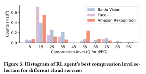
In Figure 5, for Face++ and Amazon Rekognition, the agent’s choices are mostly around compression level = 15, but for Baidu Vision, the agent’s choices are distributed more evenly. Therefore, the backend strategy really affects the choice for the optimal compression level.
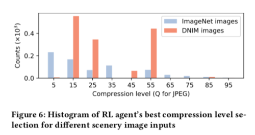
In figure 6, we will see how the agent's behaviour in selecting the optimal compression level changes for different datasets. The two datasets, ImageNet and DNIM present different contextual sceneries. The images mostly taken at daytime were randomly selected from ImageNet and the images mostly taken at the night time were selected from DNIM. The figure 6 shows that for DNiM images, the agent's choices are mostly concentrated in relatively high compression levels, whereas for ImageNet dataset, the agent's choices are distributed more evenly.
Results
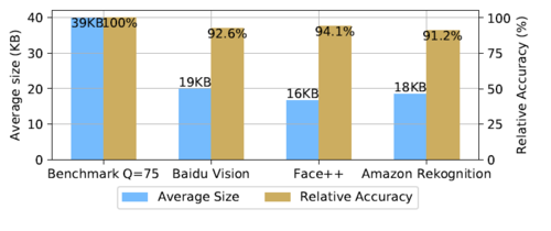
The authors reported in Figure 3, 3 different cloud services compared to the benchmark images. It is shown that more than the half of the upload size while roughly preserving the top-5 accuracy calculated by using A with an average of 7% proving the efficiency of the design. In Figure 4, it shows the inference-estimate-retain mechanism as the x-axis indicates steps, while [math]\displaystyle{ \Delta }[/math] mark on [math]\displaystyle{ x }[/math]-axis is reveal as a change in the scenery. In Figure 4, the estimating probability [math]\displaystyle{ p_{\rm est} }[/math] and the accuracy are inversely proportion as the accuracy drops below the initial value the [math]\displaystyle{ p_{\rm est} }[/math] increase adaptive as it considers the accuracy metric [math]\displaystyle{ \mathcal{A}_c }[/math] each action [math]\displaystyle{ c }[/math] making the average accuracy to decrease in the next estimations. At the red vertical line, the scenery started to change and [math]\displaystyle{ Q }[/math] Network start to retrain to adapt the the agent on the current scenery. At retrain stage, the output result is always use from the reference image's prediction label [math]\displaystyle{ \vec{y}_{\rm ref} }[/math]. Also, they plotted the scaled uploading data size of the proposed algorithm and the overhead data size for the benchmark is shown in the inference stage. After the average accuracy became stable and high, the transmission is reduced by decreasing the [math]\displaystyle{ p_{\rm est} }[/math] value. As a result, [math]\displaystyle{ p_{\rm est} }[/math] and [math]\displaystyle{ \mathcal{A} }[/math] will be always equal to 1. During this stage, the uploaded file is more than the conventional benchmark. In the inference stage, the uploaded size is halved as shown in both Figures 3, 4.
Conclusion
Most of the research focused on modifying the deep learning model instead of dealing with the currently available approaches. The authors succeed in defining the compression level for each uploaded image to decrease the size and maintain the top-5 accuracy in a robust manner even the scenery is changed. In my opinion, Eq. \eqref{eq:accuracy} is not defined well as I found it does not really affect the reward function. Also, they did not use the whole validation set from ImageNet which raises the question of what is the higher file size that they considered from in the mention current set. In addition, if they considered the whole data set, should we expect the same performance for the mechanism.
Critiques
The authors used a pre-trained model as a feature extractor to select a Quality Factor (QF) for the JPEG. I think what would be missing that they did not report the distribution of each of their span of QFs as it is important to understand which one is expected to contribute more. In my video, I have done one experiment using Inception-V3 to understand if it is possible to get better accuracy. I found that it is possible by using the inception model as a pre-trained model to choose a lower QF, but as well known that the mobile models are shallower than the inception models which make it less complex to run on edge devices. I think it is possible to achieve at least the same accuracy or even more if we replaced the mobile model with the inception. Another point, the authors did not run their approach on a complete database like ImageNet, they only included a part of two different datasets. I know they might have limitations in the available datasets to test like CIFARs, as they are not totally comparable from the resolution perspective for the real online computer vision services work with higher resolutions.
Source Code
References
[1]