stat841f14
Data Visualization (Fall 2014)
Principal Components Analysis (PCA) (Lecture: Sep. 10, 2014)
Introduction
Principal Component Analysis (PCA), first invented by Karl Pearson in 1901, is a statistical technique for data analysis. Its main purpose is to reduce the dimensionality of the data.
Suppose there is a set of data points in a p-dimensional space. PCA’s goal is to find a linear subspace with lower dimensionality q (q [math]\displaystyle{ \leq }[/math] p), such that it contains as many as possible of data points. In other words, PCA aims to reduce the dimensionality of the data, while preserving its information (or minimizing the loss of information). Information comes from variation. For example, if all data points have the same value along one dimension, that dimension does not carry any information. So, to preserve information, the subspace need to contain components (or dimensions) along which, data has its most variability. However, finding a linear subspace with lower dimensionality which include all data points is not possible in practical problems and loss of information is inevitable. But, we try to reduce this loss and capture most of the features of data.
Figure below, demonstrates an example of PCA. Data is transformed from original 3D space to 2D coordinate system where each coordiante is a principal component.
-
Data in original Space
-
Extraction of the principal components
-
Reduction of dimensionality by keeping the first two principal components and removing the third one
PCA Plot example
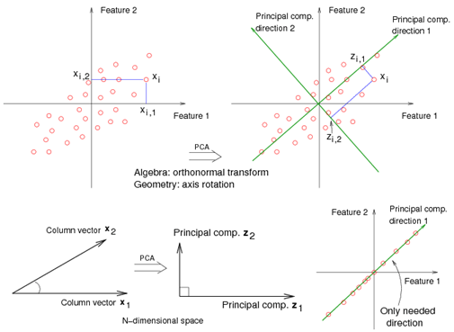
For example<ref> https://onlinecourses.science.psu.edu/stat857/sites/onlinecourses.science.psu.edu.stat857/files/lesson05/PCA_plot.gif </ref>, in the top left corner of the image, the point [math]\displaystyle{ x_1 }[/math] showed in two-dimensional and it's coordinates are [math]\displaystyle{ (x_1, 1) }[/math] and [math]\displaystyle{ (x_1, 2) }[/math]
All the red points in the plot represented by their projected values on the two original coordinators (Feature 1, Feature 2).
In PCA technique, it uses new coordinators (showed in green). As coordinate system changed, the points also are shown by their new pair of coordinate values for example [math]\displaystyle{ (z_1, 1) }[/math] and [math]\displaystyle{ (z_1, 2) }[/math]. These values are determined by original vector, and the relation between the rotated coordinates and the original ones.
In the original coordinates the two vectors [math]\displaystyle{ x_1 }[/math] and [math]\displaystyle{ x_2 }[/math] are not linearly uncorrelated. In other words, after applying PCA, if there are two principal component, and use those as the new coordinates, then it is guaranteed that the data along the two coordinates have correlation = 0
By rotating the coordinates we performed an orthonormal transform on the data. After the transform, the correlation is removed - which is the whole point of PCA.
As an example of an extreme case where all of the points lie on a straight line, which in the original coordinates system it is needed two coordinates to describe these points.
In short, after rotating the coordinates, we need only one coordinate and clearly the value on the other one is always zero. This example shows PCA's dimension reduction in an extreme case while in real world points may not fit exactly on a line, but only approximately.
PCA applications
As mentioned, PCA is a method to reduce data dimension if possible to principal components such that those PCs cover as much data variation as possible. This technique is useful in different type of applications which involve data with a huge dimension like Data pre-processing, neuroscience, Computer graphics, meteorology, oceanography, gene expression, economics, and finance among of all other applications.
Data usually is represented by lots of variables. In data preprocessing, PCA is a technique to select a subset of variables in order to figure our best model for data. In neuroscience, PCA used to identify the specific properties of a stimulus that increase a neuron’s probability of generating an action potential.
Figures below show some example of PCA in real world applications. Click to enlarge.
-
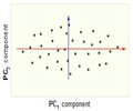
Finding two principal components of original data in 2D space. Components of data are highly correlated in original space. So they can be substituted by just one principal component, PC1, which has more than %99 of total variance of data.
-
PCA in Neuroscience. Data in different classes in 3 dimensional space is mapped to a 2 dimensional space using PCA. The mapped data is clearly linearly sparable.
Mathematical Details
PCA is a transformation from original space to a linear subspace with a new coordinate system. Each coordinate of this subspace is called a Principle Component. First principal component is the coordinate of this system along which the data points has the maximum variation. That is, if we project the data points along this coordinate, maximum variance of data is obtained (compared to any other vector in original space). Second principal component is the coordinate in the direction of the second greatest variance of the data, and so on.
Lets denote the basis of original space by [math]\displaystyle{ \mathbf{v_1} }[/math], [math]\displaystyle{ \mathbf{v_2} }[/math], ... , [math]\displaystyle{ \mathbf{v_p} }[/math]. Our goal is to find the principal components (coordinate of the linear subspace), denoted by [math]\displaystyle{ \mathbf{u_1} }[/math], [math]\displaystyle{ \mathbf{u_2} }[/math], ... , [math]\displaystyle{ \mathbf{u_q} }[/math] in the hope that [math]\displaystyle{ q \leq }[/math] p. First, we would like to obtain the first principal component [math]\displaystyle{ \mathbf{u_1} }[/math] or the components in the direction of maximum variance. This component can be treated as a vector in the original space and so is written as a linear combination of the basis in original space.
[math]\displaystyle{ \mathbf{u_1}=w_1\mathbf{v_1}+w_2\mathbf{v_2}+...+w_p\mathbf{v_p} }[/math]
Vector [math]\displaystyle{ \mathbf{w} }[/math] contains the weight of each basis in this combination.
[math]\displaystyle{ \mathbf{w}=\begin{bmatrix} w_1\\w_2\\w_3\\...\\w_p \end{bmatrix} }[/math]
Suppose we have n data points in the original space. We represent each data points by [math]\displaystyle{ \mathbf{x_1} }[/math], [math]\displaystyle{ \mathbf{x_2} }[/math], ..., [math]\displaystyle{ \mathbf{x_n} }[/math]. Projection of each point [math]\displaystyle{ \mathbf{x_i} }[/math] on the [math]\displaystyle{ \mathbf{u_1} }[/math] is [math]\displaystyle{ \mathbf{w}^T\mathbf{x_i} }[/math].
Let [math]\displaystyle{ \mathbf{S} }[/math] be the covariance matrix of data points in original space. The variance of the projected data points, denoted by [math]\displaystyle{ \Phi }[/math] is
[math]\displaystyle{ \Phi = Var(\mathbf{w}^T \mathbf{x_i}) = \mathbf{w}^T \mathbf{S} \mathbf{w} }[/math]
we would like to maximize [math]\displaystyle{ \Phi }[/math] over all set of vectors [math]\displaystyle{ \mathbf{w} }[/math] in original space. But, this problem is not yet well-defined, because for any choice of [math]\displaystyle{ \mathbf{w} }[/math], we can increase [math]\displaystyle{ \Phi }[/math] by simply multiplying [math]\displaystyle{ \mathbf{w} }[/math] in a positive scalar. So, we add the following constraint to the problem to bound the length of vector [math]\displaystyle{ \mathbf{w} }[/math]:
[math]\displaystyle{ max \Phi = \mathbf{w}^T \mathbf{S} \mathbf{w} }[/math]
subject to : [math]\displaystyle{ \mathbf{w}^T \mathbf{w} =1 }[/math]
Using Lagrange Multiplier technique we have:
[math]\displaystyle{ L(\mathbf{w} , \lambda ) = \mathbf{w}^T \mathbf{S} \mathbf{w} - \lambda (\mathbf{w}^T \mathbf{w} - 1 ) }[/math]
By taking derivative of [math]\displaystyle{ L }[/math] w.r.t. primary variable [math]\displaystyle{ \mathbf{w} }[/math] we have:
[math]\displaystyle{ \frac{\partial L}{\partial \mathbf{w}}=( \mathbf{S}^T + \mathbf{S})\mathbf{w} -2\lambda\mathbf{w}= 2\mathbf{S}\mathbf{w} -2\lambda\mathbf{w}= 0 }[/math]
Note that [math]\displaystyle{ \mathbf{S} }[/math] is symmetric so [math]\displaystyle{ \mathbf{S}^T = \mathbf{S} }[/math].
So, we have:
[math]\displaystyle{ \mathbf{S} \mathbf{w} = \lambda\mathbf{w} }[/math].
So [math]\displaystyle{ \mathbf{w} }[/math] is the eigenvector and [math]\displaystyle{ \lambda }[/math] is the eigenvalue of the matrix [math]\displaystyle{ \mathbf{S} }[/math] .(Taking derivative of [math]\displaystyle{ L }[/math] w.r.t. [math]\displaystyle{ \lambda }[/math] just regenerate the constraint of the optimization problem.)
By multiplying both sides of the above equation to [math]\displaystyle{ \mathbf{w}^T }[/math] and considering the constraint, we obtain:
[math]\displaystyle{ \Phi = \mathbf{w}^T \mathbf{S} \mathbf{w} = \mathbf{w}^T \lambda \mathbf{w} = \lambda \mathbf{w}^T \mathbf{w} = \lambda }[/math]
The interesting result is that objective function is equal to eigenvalue of the covariance matrix. So, to obtain the first principle component, which maximizes the objective function, we just need the eigenvector corresponding to the largest eigenvalue of [math]\displaystyle{ \mathbf{S} }[/math]. Subsequently, the second principal component is the eigenvector corresponding to the second largest eigenvalue, and so on.
Principal Component Extraction using Singular Value Decomposition
Singular Value Decomposition (SVD), is a well-known way to decompose any kind of matrix [math]\displaystyle{ \mathbf{A} }[/math] (m by n) into three useful matrices.
[math]\displaystyle{ \mathbf{A} = \mathbf{U}\mathbf{\Sigma}\mathbf{V}^T }[/math].
where [math]\displaystyle{ \mathbf{U} }[/math] is m by m unitary matrix, [math]\displaystyle{ \mathbf{UU^T} = I_m }[/math], each column of [math]\displaystyle{ \mathbf{U} }[/math] is an eigenvector of [math]\displaystyle{ \mathbf{AA^T} }[/math]
[math]\displaystyle{ \mathbf{V} }[/math] is n by n unitary matrix, [math]\displaystyle{ \mathbf{VV^T} = I_n }[/math], each column of [math]\displaystyle{ \mathbf{V} }[/math] is an eigenvector of [math]\displaystyle{ \mathbf{A^TA} }[/math]
[math]\displaystyle{ \mathbf{\Sigma} }[/math] is m by n diagonal matrix, non-zero elements of this matrix are square roots of eigenvalues of [math]\displaystyle{ \mathbf{AA^T} }[/math].
Now, comparing the concepts of PCA and SVD, one may find out that we can perform PCA using SVD.
Lets construct a matrix p by n with our n data points such that each column of this matrix represent one data point in p-dimensional space:
[math]\displaystyle{ \mathbf{X} = [\mathbf{x_1} \mathbf{x_2} .... \mathbf{x_n} ] }[/math]
and make another matrix [math]\displaystyle{ \mathbf{X}^* }[/math] simply by subtracting the mean of data points from [math]\displaystyle{ \mathbf{X} }[/math].
[math]\displaystyle{ \mathbf{X}^* = \mathbf{X} - \mu_X }[/math]
Then we will get a zero-mean version of our data points for which [math]\displaystyle{ \mathbf{X^*} \mathbf{X^{*^T}} }[/math] is the covariance matrix.
So, [math]\displaystyle{ \mathbf{\Sigma} }[/math] and [math]\displaystyle{ \mathbf{U} }[/math] give us the eigenvalues and corresponding eigenvectors of covariance matrix, respectively. We can then easily extract the desired principal components.
MATLAB Example
In this example we use different pictures of a man's face with different facial expressions. But, these pictures are noisy. So the face is not easily recognizable. The data set consists of 1965 pictures each 20 by 28. So dimensionality is 20*28= 560.
Our goal is to remove noise using PCA and of course by means of SVD function in matlab. We know that noise is not the main feature that makes these pictures look different. So noise is among least variance components. We first extract the principal components and then remove those which correspond to the least values of eigenvalues of covariance matrix. Here, eigenvalues are sorted in a descending order from column to column of matrix S. So, for example first column of matrix U which corresponds to first element in S, is the first principal component.
We then reconstruct the picture using first d principal components. If d is too large, we can not completely remove the noise. If it is too small, we will loose some information from original data, for example we may loose the facial expression (smile, sadness and etc.). We can change d until we achieve a reasonable balance between noise reduction and information loss.
 >> % loading the noisy data, file "noisy" stores our variable X which contains the pictures
 >> load noisy;
 >>
 >>
 >> % show an sample image in column 1 of matrix X
 >> imagesc(reshape(X(:,1),20,28)')
 >>
 >> % set the color of image to grayscale
 >> colormap gray
 >>
 >> % perform SVD, if X matrix if full rank, will obtain 560 PCs
 >> [U S V] = svd(X);
 >>
 >> d= 10;
 >>
 >> % reconstruct X using only the first d principal components and removing noise
 >> XX = U(:, 1:d)* S(1:d,1:d)*U(:,1:d)' ;
 >>
 >> % show image in column 1 of XX which is a noise reduced version
 >> imagesc(reshape(XX(:,1),20,28)')


