stat841f10: Difference between revisions
| Line 157: | Line 157: | ||
== '''Linear and Quadratic Discriminant Analysis''' == | == '''Linear and Quadratic Discriminant Analysis''' == | ||
{{Cleanup|date=September 2010|reason=The derivation of the Bayes classifier's decision boundary in the two-classes case needs to be checked since I am not sure if it is entirely correct}} | {{Cleanup|date=September 2010|reason=The derivation of the Bayes classifier's decision boundary in the two-classes case needs to be checked over since I am not sure if it is entirely correct}} | ||
First, we shall limit ourselves to the case where there are two classes, i.e. <math>\, \mathcal{Y}=\{0, 1\}</math>. In the above discussion, we introduced the Bayes classifier's ''decision boundary'' <math>\,D(h)=\{x: P(Y=1|X=x)=P(Y=0|X=x)\}</math>, which represents a separating [http://en.wikipedia.org/wiki/Hyperplane hyperplane] that determines the class of any new data input depending on which side of the decision boundary the input lies in. Now, we shall look at how to derive the decision boundary for the Bayes classifier under certain assumptions of the data. [http://en.wikipedia.org/wiki/Linear_discriminant_analysis Linear discriminant analysis (LDA)] and [http://en.wikipedia.org/wiki/Quadratic_classifier#Quadratic_discriminant_analysis quadratic discriminant analysis (QDA)] are two of the most well-known derivations of the Bayes classifier's decision boundary, and shall look at each of them in turn. | First, we shall limit ourselves to the case where there are two classes, i.e. <math>\, \mathcal{Y}=\{0, 1\}</math>. In the above discussion, we introduced the Bayes classifier's ''decision boundary'' <math>\,D(h)=\{x: P(Y=1|X=x)=P(Y=0|X=x)\}</math>, which represents a separating [http://en.wikipedia.org/wiki/Hyperplane hyperplane] that determines the class of any new data input depending on which side of the decision boundary the input lies in. Now, we shall look at how to derive the decision boundary for the Bayes classifier under certain assumptions of the data. [http://en.wikipedia.org/wiki/Linear_discriminant_analysis Linear discriminant analysis (LDA)] and [http://en.wikipedia.org/wiki/Quadratic_classifier#Quadratic_discriminant_analysis quadratic discriminant analysis (QDA)] are two of the most well-known derivations of the Bayes classifier's decision boundary, and shall look at each of them in turn. | ||
| Line 179: | Line 179: | ||
\mu_1-\mu_0^\top\Sigma^{-1}\mu_0 - 2x^\top\Sigma^{-1}(\mu_1-\mu_0) \right)=0</math> (canceling out like terms and factoring). | \mu_1-\mu_0^\top\Sigma^{-1}\mu_0 - 2x^\top\Sigma^{-1}(\mu_1-\mu_0) \right)=0</math> (canceling out like terms and factoring). | ||
<math>\,\Rightarrow -2\log(\frac{\pi_1}{\pi_0})+\mu_1^\top\Sigma^{-1}\mu_1+\mu_0^\top\Sigma^{-1}\mu_0 + 2x^\top\Sigma^{-1}(\mu_1-\mu_0)=0</math> | |||
| Line 186: | Line 187: | ||
Revision as of 18:52, 28 September 2010
Editor sign up
Classfication-2010.09.21
Classification
{{
Template:namespace detect
| type = style | image = | imageright = | style = | textstyle = | text = This article may require cleanup to meet Wikicoursenote's quality standards. The specific problem is: I think there are different viewes. Some people name the supervised learning, "classification" and the unsupervised learning,"clustering" . But the other ones are just calling the clustering, "unsupervised classification", like http://www.yale.edu/ceo/Projects/swap/landcover/Unsupervised_classification.htm and other groups which could be found by a google search. Finally, I think It is good to be cleared here.. Please improve this article if you can. (28 September 2010) | small = | smallimage = | smallimageright = | smalltext = }} Statistical classification, or simply known as classification, is an area of supervised learning that addresses the problem of how to systematically assign unlabeled (classes unknown) novel data to their labels (classes or groups or types) by using knowledge of their features (characteristics or attributes) that are obtained from observation and/or measurement. A classifier is a specific technique or method for performing classification. To classify new data, a classifier first uses labeled (classes are known) training data to train a model, and then it uses a function known as its classification rule to assign a label to each new data input after feeding the input's known feature values into the model to determine how much the input belongs to each class.
Classification has been an important task for people and society since the beginnings of history. According to this link, the earliest application of classification in human society was probably done by prehistory peoples for recognizing which wild animals were beneficial to people and which one were harmful, and the earliest systematic use of classification was done by the famous Greek philosopher Aristotle when he, for example, grouped all living things into the two groups of plants and animals. Classification is generally regarded as one of four major areas of statistics, with the other three major areas being regression regression, clustering, and dimensionality reduction (feature extraction or manifold learning).
In classical statistics, classification techniques were developed to learn useful information using small data sets where there is usually not enough of data. When machine learning was developed after the application of computers to statistics, classification techniques were developed to work with very large data sets where there is usually too many data. A major challenge facing data mining using machine learning is how to efficiently find useful patterns in very large amounts of data. An interesting quote that describes this problem quite well is the following one made by the retired Yale University Librarian Rutherford D. Rogers.
       "We are drowning in information and starving for knowledge."
                                                         - Rutherford D. Rogers
In the Information Age, machine learning when it is combined with efficient classification techniques can be very useful for data mining using very large data sets. This is most useful when the structure of the data is not well understood but the data nevertheless exhibit strong statistical regularity. Areas in which machine learning and classification have been successfully used together include search and recommendation (e.g. Google, Amazon), automatic speech recognition and speaker verification, medical diagnosis, analysis of gene expression, drug discovery etc.
The formal mathematical definition of classification is as follows:
Definition: Classification is the prediction of a discrete random variable [math]\displaystyle{ \mathcal{Y} }[/math] from another random variable [math]\displaystyle{ \mathcal{X} }[/math], where [math]\displaystyle{ \mathcal{Y} }[/math] represents the label assigned to a new data input and [math]\displaystyle{ \mathcal{X} }[/math] represents the known feature values of the input.
A set of training data used by a classifier to train its model consists of [math]\displaystyle{ \,n }[/math] independently and identically distributed (i.i.d) ordered pairs [math]\displaystyle{ \,\{(X_{1},Y_{1}), (X_{2},Y_{2}), \dots , (X_{n},Y_{n})\} }[/math], where the values of the [math]\displaystyle{ \,ith }[/math] training input's feature values [math]\displaystyle{ \,X_{i} = (\,X_{i1}, \dots , X_{id}) \in \mathcal{X} \subset \mathbb{R}^{d} }[/math] is a d-dimensional vector and the label of the [math]\displaystyle{ \, ith }[/math] training input is [math]\displaystyle{ \,Y_{i} \in \mathcal{Y} }[/math] that takes a finite number of values. The classification rule used by a classifier has the form [math]\displaystyle{ \,h: \mathcal{X} \mapsto \mathcal{Y} }[/math]. After the model is trained, each new data input whose feature values is [math]\displaystyle{ \,X \in \mathcal{X}, }[/math] is given the label [math]\displaystyle{ \,\hat{Y}=h(X) \in \mathcal{Y} }[/math].
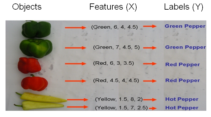
As an example, if we would like to classify some vegetables and fruits, then our training data might look something like the one shown in the following picture from Professor Ali Ghodsi's Fall 2010 STAT 841 slides.
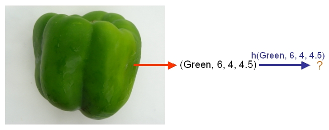
After we have selected a classifier and then built our model using our training data, we could use the classifier's classification rule [math]\displaystyle{ \ h }[/math] to classify any newly-given vegetable or fruit such as the one shown in the following picture from Professor Ali Ghodsi's Fall 2010 STAT 841 slides after first obtaining its feature values.
As another example, suppose we wish to classify newly-given fruits into apples and oranges by considering three features of a fruit that comprise its color, its diameter, and its weight. After selecting a classifier and constructing a model using training data [math]\displaystyle{ \,\{(X_{color, 1}, X_{diameter, 1}, X_{weight, 1}, Y_{1}), \dots , (X_{color, n}, X_{diameter, n}, X_{weight, n}, Y_{n})\} }[/math], we could then use the classifier's classification rule [math]\displaystyle{ \,h }[/math] to assign any newly-given fruit having known feature values [math]\displaystyle{ \,X = (\,X_{color}, X_{diameter} , X_{weight}) \in \mathcal{X} \subset \mathbb{R}^{3} }[/math] the label [math]\displaystyle{ \,\hat{Y}=h(X) \in \mathcal{Y} }[/math], where [math]\displaystyle{ \mathcal{Y}=\{\mathrm{apple}, \mathrm{orange}\} }[/math].
Error rate
The true error rate' [math]\displaystyle{ \,L(h) }[/math] of a classifier having classification rule [math]\displaystyle{ \,h }[/math] is defined as the probability that [math]\displaystyle{ \,h }[/math] does not correctly classify any new data input, i.e., it is defined as [math]\displaystyle{ \,L(h)=P(h(X) \neq Y) }[/math]. Here, [math]\displaystyle{ \,X \in \mathcal{X} }[/math] and [math]\displaystyle{ \,Y \in \mathcal{Y} }[/math] are the known feature values and the true class of that input, respectively.
The empirical error rate (or training error rate) of a classifier having classification rule [math]\displaystyle{ \,h }[/math] is defined as the frequency at which [math]\displaystyle{ \,h }[/math] does not correctly classify the data inputs in the training set, i.e., it is defined as [math]\displaystyle{ \,\hat{L}_{n} = \frac{1}{n} \sum_{i=1}^{n} I(h(X_{i}) \neq Y_{i}) }[/math], where [math]\displaystyle{ \,I }[/math] is an indicator variable and [math]\displaystyle{ \,I = \left\{\begin{matrix} 1 &\text{if } h(X_i) \neq Y_i \\ 0 &\text{if } h(X_i) = Y_i \end{matrix}\right. }[/math]. Here, [math]\displaystyle{ \,X_{i} \in \mathcal{X} }[/math] and [math]\displaystyle{ \,Y_{i} \in \mathcal{Y} }[/math] are the known feature values and the true class of the [math]\displaystyle{ \,ith }[/math] training input, respectively.
Bayes Classifier
After training its model using training data, the Bayes classifier classifies any new data input in two steps. First, it uses the input's known feature values and the Bayes formula to calculate the input's posterior probability of belonging to each class. Then, it uses its classification rule to place the input into its most-probable class, which is the one associated with the input's largest posterior probability.
In mathematical terms, for a new data input having feature values [math]\displaystyle{ \,(X = x)\in \mathcal{X} }[/math], the Bayes classifier labels the input as [math]\displaystyle{ (Y = y) \in \mathcal{Y} }[/math], such that the input's posterior probability [math]\displaystyle{ \,P(Y = y|X = x) }[/math] is maximum over all the members of [math]\displaystyle{ \mathcal{Y} }[/math].
Suppose there are [math]\displaystyle{ \,k }[/math] classes and we are given a new data input having feature values [math]\displaystyle{ \,X=x }[/math]. The following derivation shows how the Bayes classifier finds the input's posterior probability [math]\displaystyle{ \,P(Y = y|X = x) }[/math] of belonging to each class [math]\displaystyle{ (Y = y) \in \mathcal{Y} }[/math].
- [math]\displaystyle{ \begin{align} P(Y=y|X=x) &= \frac{P(X=x|Y=y)P(Y=y)}{P(X=x)} \\ &=\frac{P(X=x|Y=y)P(Y=y)}{\Sigma_{\forall i \in \mathcal{Y}}P(X=x|Y=i)P(Y=i)} \end{align} }[/math]
Here, [math]\displaystyle{ \,P(Y=y|X=x) }[/math] is known as the posterior probability as mentioned above, [math]\displaystyle{ \,P(Y=y) }[/math] is known as the prior probability, [math]\displaystyle{ \,P(X=x|Y=y) }[/math] is known as the likelihood, and [math]\displaystyle{ \,P(X=x) }[/math] is known as the evidence.
In the special case where there are two classes, i.e., [math]\displaystyle{ \, \mathcal{Y}=\{0, 1\} }[/math], the Bayes classifier makes use of the function [math]\displaystyle{ \,r(x)=P\{Y=1|X=x\} }[/math] which is the prior probability of a new data input having feature values [math]\displaystyle{ \,X=x }[/math] belonging to the class [math]\displaystyle{ \,Y = 1 }[/math]. Following the above derivation for the posterior probabilities of a new data input, the Bayes classifier calculates [math]\displaystyle{ \,r(x) }[/math] as follows:
- [math]\displaystyle{ \begin{align} r(x)&=P(Y=1|X=x) \\ &=\frac{P(X=x|Y=1)P(Y=1)}{P(X=x)}\\ &=\frac{P(X=x|Y=1)P(Y=1)}{P(X=x|Y=1)P(Y=1)+P(X=x|Y=0)P(Y=0)} \end{align} }[/math]
The Bayes classifier's classification rule [math]\displaystyle{ \,h^*: \mathcal{X} \mapsto \mathcal{Y} }[/math], then, is
- [math]\displaystyle{ \, h^*(x)= \left\{\begin{matrix} 1 &\text{if } \hat r(x)\gt \frac{1}{2} \\ 0 &\text{if } \mathrm{otherwise} \end{matrix}\right. }[/math].
Here, [math]\displaystyle{ \,x }[/math] is the feature values of a new data input and [math]\displaystyle{ \hat r(x) }[/math] is the estimated value of the function [math]\displaystyle{ \,r(x) }[/math] given by the Bayes classifier's model after feeding [math]\displaystyle{ \,x }[/math] into the model. Still in this special case of two classes, the Bayes classifier's decision boundary is defined as the set [math]\displaystyle{ \,D(h)=\{x: P(Y=1|X=x)=P(Y=0|X=x)\} }[/math]. The decision boundary [math]\displaystyle{ \,D(h) }[/math] essentially combines together the trained model and the decision function [math]\displaystyle{ \,h }[/math], and it is used by the Bayes classifier to assign any new data input to a label of either [math]\displaystyle{ \,Y = 0 }[/math] or [math]\displaystyle{ \,Y = 1 }[/math] depending on which side of the decision boundary the input lies in. From this decision boundary, it is easy to see that, in the case where there are two classes, the Bayes classifier's classification rule can be re-expressed as
- [math]\displaystyle{ \, h^*(x)= \left\{\begin{matrix} 1 &\text{if } P(Y=1|X=x)\gt P(Y=0|X=x) \\ 0 &\text{if } \mathrm{otherwise} \end{matrix}\right. }[/math].
Bayes Classification Rule Optimality Theorem
- The Bayes classifier is the optimal classifier in that it produces the least possible probability of misclassification for any given new data input, i.e., for any other classifier having classification rule [math]\displaystyle{ \,h }[/math], it is always true that [math]\displaystyle{ \,L(h^*(x)) \le L(h(x)) }[/math]. Here, [math]\displaystyle{ \,L }[/math] represents the true error rate, [math]\displaystyle{ \,h^* }[/math] is the Bayes classifier's classification rule, and [math]\displaystyle{ \,x }[/math] is any given data input's feature values.
Although the Bayes classifier is optimal in the theoretical sense, other classifiers may nevertheless outperform it in practice. The reason for this is that various components which make up the Bayes classifier's model, such as the likelihood and prior probabilities, must either be estimated using training data or be guessed with a certain degree of belief, as a result, their estimated values in the trained model may deviate quite a bit from their true population values and this ultimately can cause the posterior probabilities to deviate quite a bit from their true population values. A rather detailed proof of this theorem is available here.
Defining the classification rule:
In the special case of two classes, the Bayes classifier can use three main approaches to define its classification rule [math]\displaystyle{ \,h }[/math]:
- 1) Empirical Risk Minimization: Choose a set of classifiers [math]\displaystyle{ \mathcal{H} }[/math] and find [math]\displaystyle{ \,h^*\in \mathcal{H} }[/math] that minimizes some estimate of the true error rate [math]\displaystyle{ \,L(h) }[/math].
- 2) Regression: Find an estimate [math]\displaystyle{ \hat r }[/math] of the function [math]\displaystyle{ x }[/math] and define
- [math]\displaystyle{ \, h(x)= \left\{\begin{matrix} 1 &\text{if } \hat r(x)\gt \frac{1}{2} \\ 0 &\text{if } \mathrm{otherwise} \end{matrix}\right. }[/math].
- 3) Density Estimation: Estimate [math]\displaystyle{ \,P(X=x|Y=0) }[/math] from the [math]\displaystyle{ \,X_{i} }[/math]'s for which [math]\displaystyle{ \,Y_{i} = 0 }[/math], estimate [math]\displaystyle{ \,P(X=x|Y=1) }[/math] from the [math]\displaystyle{ \,X_{i} }[/math]'s for which [math]\displaystyle{ \,Y_{i} = 1 }[/math], and estimate [math]\displaystyle{ \,P(Y = 1) }[/math] as [math]\displaystyle{ \,\frac{1}{n} \sum_{i=1}^{n} Y_{i} }[/math]. Then, calculate [math]\displaystyle{ \,\hat r(x) = \hat P(Y=1|X=x) }[/math] and define
- [math]\displaystyle{ \, h(x)= \left\{\begin{matrix} 1 &\text{if } \hat r(x)\gt \frac{1}{2} \\ 0 &\text{if } \mathrm{otherwise} \end{matrix}\right. }[/math].
Typically, the Bayes classifier uses approach 3 to define its classification rule. These three approaches can easily be generalized to the case where the number of classes exceeds two.
Multi-class classification:
Suppose there are [math]\displaystyle{ \,k }[/math] classes, where [math]\displaystyle{ \,k \ge 2 }[/math].
In the above discussion, we introduced the Bayes formula for this general case:
- [math]\displaystyle{ \begin{align} P(Y=y|X=x) &=\frac{P(X=x|Y=y)P(Y=y)}{\Sigma_{\forall i \in \mathcal{Y}}P(X=x|Y=i)P(Y=i)} \end{align} }[/math]
which can re-worded as:
- [math]\displaystyle{ \begin{align} P(Y=y|X=x) &=\frac{f_y(x)\pi_y}{\Sigma_{\forall i \in \mathcal{Y}} f_i(x)\pi_i} \end{align} }[/math]
Here, [math]\displaystyle{ \,f_y(x) = P(X=x|Y=y) }[/math] is known as the likelihood function and [math]\displaystyle{ \,\pi_y = P(Y=y) }[/math] is known as the prior probability.
In the general case where there are at least two classes, the Bayes classifier uses the following theorem to assign any new data input having feature values [math]\displaystyle{ \,x }[/math] into one of the [math]\displaystyle{ \,k }[/math] classes.
Theorem
- Suppose that [math]\displaystyle{ \mathcal{Y}= \{1, \dots, k\} }[/math], where [math]\displaystyle{ \,k \ge 2 }[/math]. Then, the optimal classification rule is [math]\displaystyle{ \,h^*(x) = argmax_{i} P(Y=i|X=x) }[/math], where [math]\displaystyle{ \,i \in \{1, \dots, k\} }[/math].
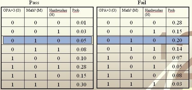
Example: We are going to predict if a particular student will pass STAT 441/841. There are two classes represented by [math]\displaystyle{ \, \mathcal{Y}\in \{ 0,1 \} }[/math], where 1 refers to pass and 0 refers to fail. Suppose that the prior probabilities are estimated or guessed to be [math]\displaystyle{ \,\hat P(Y = 1) = \hat P(Y = 0) = 0.5 }[/math]. We have data on past student performances, which we shall use to train the model. For each student, we know the following:
- Whether or not the student’s GPA was greater than 3.0 (G).
- Whether or not the student had a strong math background (M).
- Whether or not the student was a hard worker (H).
- Whether or not the student passed or failed the course.
These known data are summarized in the following tables:
For each student, his/her feature values is [math]\displaystyle{ \, x = \{G, M, H\} }[/math] and his or her class is [math]\displaystyle{ \, y \in \{0, 1\} }[/math].
Suppose there is a new student having feature values [math]\displaystyle{ \, x = \{0, 1, 0\} }[/math], and we would like to predict whether he/she would pass the course. [math]\displaystyle{ \,\hat r(x) }[/math] is found as follows:
[math]\displaystyle{ \, \hat r(x) = P(Y=1|X =(0,1,0))=\frac{P(X=(0,1,0)|Y=1)P(Y=1)}{P(X=(0,1,0)|Y=0)P(Y=0)+P(X=(0,1,0)|Y=1)P(Y=1)}=\frac{0.025}{0.125}=0.2\lt \frac{1}{2}. }[/math]
The Bayes classifier assigns the new student into the class [math]\displaystyle{ \, h^*(x)=0 }[/math]. Therefore, we predict that the new student would fail the course.
Bayesian vs. Frequentist
The Bayesian view of probability and the frequentist view of probability are the two major schools of thought in the field of statistics regarding how to interpret the probability of an event.
The Bayesian view of probability states that, for any event E, event E has a prior probability that represents how believable event E would occur prior to knowing anything about any other event whose occurrence could have an impact on event E's occurrence. Theoretically, this prior probability is a belief that represents the baseline probability for event E's occurrence. In practice, however, event E's prior probability is unknown, and therefore it must either be guessed at or be estimated using a sample of available data. After obtaining a guessed or estimated value of event E's prior probability, the Bayesian view holds that the probability, that is, the believability, of event E's occurrence can always be made more accurate should any new information regarding events that are relevant to event E become available. The Bayesian view also holds that the accuracy for the estimate of the probability of event E's occurrence is higher as long as there are more useful information available regarding events that are relevant to event E. The Bayesian view therefore holds that there is no intrinsic probability of occurrence associated with any event. If one adherers to the Bayesian view, one can then, for instance, predict tomorrow's weather as having a probability of, say, [math]\displaystyle{ \,50% }[/math] for rain. The Bayes classifier as described above is a good example of a classifier developed from the Bayesian view of probability. The earliest works that lay the framework for the Bayesian view of probability is accredited to Thomas Bayes (1702–1761).
In contrast to the Bayesian view of probability, the frequentist view of probability holds that there is an intrinsic probability of occurrence associated with every event to which one can carry out many, if not an infinite number, of well-defined independent random trials. In each trial for an event, the event either occurs or it does not occur. Suppose [math]\displaystyle{ n_x }[/math] denotes the number of times that an event occurs during its trials and [math]\displaystyle{ n_t }[/math] denotes the total number of trials carried out for the event. The frequentist view of probability holds that, in the long run, where the number of trials for an event approaches infinity, one could theoretically approach the intrinsic value of the event's probability of occurrence to any arbitrary degree of accuracy, i.e., :[math]\displaystyle{ P(x) = \lim_{n_t\rightarrow \infty}\frac{n_x}{n_t}. }[/math]. In practice, however, one can only carry out a finite number of trials for an event and, as a result, the probability of the event's occurrence can only be approximated as [math]\displaystyle{ P(x) \approx \frac{n_x}{n_t} }[/math].If one adherers to the frequentist view, one cannot, for instance, predict the probability that there would be rain tomorrow, and this is because one cannot possibly carry out trials on any event that is set in the future. The founder of the frequentist school of thought is arguably the famous Greek philosopher Aristotle. In his work Rhetoric, Aristotle gave the famous line "the probable is that which for the most part happens".
More information regarding the Bayesian and the frequentist schools of thought are available here. Furthermore, an interesting and informative youtube video that explains the Bayesian and frequentist views of probability is available here.
Linear and Quadratic Discriminant Analysis
{{
Template:namespace detect
| type = style | image = | imageright = | style = | textstyle = | text = This article may require cleanup to meet Wikicoursenote's quality standards. The specific problem is: The derivation of the Bayes classifier's decision boundary in the two-classes case needs to be checked over since I am not sure if it is entirely correct. Please improve this article if you can. (September 2010) | small = | smallimage = | smallimageright = | smalltext = }}
First, we shall limit ourselves to the case where there are two classes, i.e. [math]\displaystyle{ \, \mathcal{Y}=\{0, 1\} }[/math]. In the above discussion, we introduced the Bayes classifier's decision boundary [math]\displaystyle{ \,D(h)=\{x: P(Y=1|X=x)=P(Y=0|X=x)\} }[/math], which represents a separating hyperplane that determines the class of any new data input depending on which side of the decision boundary the input lies in. Now, we shall look at how to derive the decision boundary for the Bayes classifier under certain assumptions of the data. Linear discriminant analysis (LDA) and quadratic discriminant analysis (QDA) are two of the most well-known derivations of the Bayes classifier's decision boundary, and shall look at each of them in turn.
Let us denote the likelihood [math]\displaystyle{ \ P(X=x|Y=y) }[/math] as [math]\displaystyle{ \ f_y(x) }[/math] and the prior probability [math]\displaystyle{ \ P(Y=y) }[/math] as [math]\displaystyle{ \ \pi_y }[/math].
Under the assumptions of LDA, we have: [math]\displaystyle{ \ P(X=x|Y=y) = f_y(x) = \frac{1}{ (2\pi)^{d/2}|\Sigma_k|^{1/2} }\exp\left( -\frac{1}{2} (x - \mu_k)^\top \Sigma_k^{-1} (x - \mu_k) \right) }[/math].
First, we shall examine LDA. As explained above, the Bayes classifier is optimal. However, in practice, the prior and conditional densities are not known. Under LDA, one gets around this problem by making the assumption that the data from each of the two classes are generated from a multivariate normal (Gaussian) distribution and that the two classes have the same covariance matrix [math]\displaystyle{ \, \Sigma }[/math]. Now, to solve for the Bayes classifier's decision boundary, we equate [math]\displaystyle{ \, P(Y=1|X=x) }[/math] and [math]\displaystyle{ \, P(Y=0|X=x) }[/math] and proceed from there. The derivation of the decision boundary is as follows:
- [math]\displaystyle{ \,Pr(Y=1|X=x)=Pr(Y=0|X=x) }[/math]
[math]\displaystyle{ \,\Rightarrow \frac{Pr(X=x|Y=1)Pr(Y=1)}{Pr(X=x)}=\frac{Pr(X=x|Y=0)Pr(Y=0)}{Pr(X=x)} }[/math] (using Bayes' Theorem) [math]\displaystyle{ \,\Rightarrow Pr(X=x|Y=1)Pr(Y=1)=Pr(X=x|Y=0)Pr(Y=0) }[/math] (canceling the denominators) [math]\displaystyle{ \,\Rightarrow f_1(x)\pi_1=f_0(x)\pi_0 }[/math] [math]\displaystyle{ \,\Rightarrow \frac{1}{ (2\pi)^{d/2}|\Sigma|^{1/2} }\exp\left( -\frac{1}{2} (x - \mu_1)^\top \Sigma^{-1} (x - \mu_1) \right)\pi_1=\frac{1}{ (2\pi)^{d/2}|\Sigma|^{1/2} }\exp\left( -\frac{1}{2} (x - \mu_0)^\top \Sigma^{-1} (x - \mu_0) \right)\pi_0 }[/math] [math]\displaystyle{ \,\Rightarrow \exp\left( -\frac{1}{2} (x - \mu_1)^\top \Sigma^{-1} (x - \mu_1) \right)\pi_1=\exp\left( -\frac{1}{2} (x - \mu_0)^\top \Sigma^{-1} (x - \mu_0) \right)\pi_0 }[/math] [math]\displaystyle{ \,\Rightarrow -\frac{1}{2} (x - \mu_1)^\top \Sigma^{-1} (x - \mu_1) + \log(\pi_1)=-\frac{1}{2} (x - \mu_0)^\top \Sigma^{-1} (x - \mu_0) +\log(\pi_0) }[/math] (taking the log of both sides). [math]\displaystyle{ \,\Rightarrow \log(\frac{\pi_1}{\pi_0})-\frac{1}{2}\left( x^\top\Sigma^{-1}x + \mu_1^\top\Sigma^{-1}\mu_1 - 2x^\top\Sigma^{-1}\mu_1 - x^\top\Sigma^{-1}x - \mu_0^\top\Sigma^{-1}\mu_0 + 2x^\top\Sigma^{-1}\mu_0 \right)=0 }[/math] (expanding out)
[math]\displaystyle{ \,\Rightarrow \log(\frac{\pi_1}{\pi_0})-\frac{1}{2}\left( \mu_1^\top\Sigma^{-1} \mu_1-\mu_0^\top\Sigma^{-1}\mu_0 - 2x^\top\Sigma^{-1}(\mu_1-\mu_0) \right)=0 }[/math] (canceling out like terms and factoring).
[math]\displaystyle{ \,\Rightarrow -2\log(\frac{\pi_1}{\pi_0})+\mu_1^\top\Sigma^{-1}\mu_1+\mu_0^\top\Sigma^{-1}\mu_0 + 2x^\top\Sigma^{-1}(\mu_1-\mu_0)=0 }[/math]
- [math]\displaystyle{ \begin{align} P(Y=y|X=x) &=\frac{P(X=x|Y=y)P(Y=y)}{\Sigma_{\forall y \in \mathcal{Y}}P(X=x|Y=y)P(Y=y)} \end{align} }[/math]
We will use new labels for the following equivalent formula:
- [math]\displaystyle{ \begin{align} P(Y=k|X=x) &=\frac{f_k(x)\pi_k}{\Sigma_kf_k(x)\pi_k} \end{align} }[/math]
History
The name Linear Discriminant Analysis comes from the fact that these simplifications produce a linear model, which is used to discriminate between classes. In many cases, this simple model is sufficient to provide a near optimal classification - for example, the Z-Score credit risk model, designed by Edward Altman in 1968, which is essentially a weighted LDA, revisited in 2000, has shown an 85-90% success rate predicting bankruptcy, and is still in use today.
Purpose
1 feature selection
2 which classification rule best seperate the classes
Definition
To perform LDA we make two assumptions.
- The clusters belonging to all classes each follow a multivariate normal distribution.
[math]\displaystyle{ x \in \mathbb{R}^d }[/math] [math]\displaystyle{ f_k(x)=\frac{1}{ (2\pi)^{d/2}|\Sigma_k|^{1/2} }\exp\left( -\frac{1}{2} [x - \mu_k]^\top \Sigma_k^{-1} [x - \mu_k] \right) }[/math]
where [math]\displaystyle{ \ f_k(x) }[/math] is a class conditional density
- Simplification Assumption: Each cluster has the same covariance matrix [math]\displaystyle{ \,\Sigma }[/math] equal to the covariance of [math]\displaystyle{ \Sigma_k \forall k }[/math].
We can see that this is a linear function in [math]\displaystyle{ \ x }[/math] with general form [math]\displaystyle{ \,ax+b=0 }[/math].
Actually, this linear log function shows that the decision boundary between class [math]\displaystyle{ \ k }[/math] and class [math]\displaystyle{ \ l }[/math], i.e. [math]\displaystyle{ \ P(G=k|X=x)=P(G=l|X=x) }[/math], is linear in [math]\displaystyle{ \ x }[/math]. Given any pair of classes, decision boundaries are always linear. In [math]\displaystyle{ \ d }[/math] dimensions, we separate regions by hyperplanes.
In the special case where the number of samples from each class are equal ([math]\displaystyle{ \,\pi_k=\pi_l }[/math]), the boundary surface or line lies halfway between [math]\displaystyle{ \,\mu_l }[/math] and [math]\displaystyle{ \,\mu_k }[/math]
Limitation
- LDA implicitly assumes Gaussian distribution of data.
- LDA implicitly assumes that the mean is the discriminating factor, not variance.
- LDA may overfit the data.
Notation=
Let us first introduce some new notation for the following sections.
Multi-class Classification:
Y takes on more than two values.
Recall that in the discussion of the Bayes Classifier, we introduced Bayes Formula:
- [math]\displaystyle{ \,f_k }[/math] is called the class conditional density; also referred to previously as the likelihood function. Essentially, this is the function that allows us to reason about a parameter given a certain outcome.
- [math]\displaystyle{ \,\pi_k }[/math] is called the prior probability. This is a probability distribution that represents what we know (or believe we know) about a population.
- [math]\displaystyle{ \,\Sigma_k }[/math] is the sum with respect to all [math]\displaystyle{ \,k }[/math] classes.
QDA
The concept uses a same idea as LDA of finding a boundary where the error rate for classification between classes are equal, except the assumption that each cluster has the same variance [math]\displaystyle{ \,\Sigma }[/math] equal to the mean variance of [math]\displaystyle{ \Sigma_k \forall k }[/math] is removed. We can use a hypothesis test with [math]\displaystyle{ \ H_0 }[/math]: [math]\displaystyle{ \Sigma_k \forall k }[/math]=[math]\displaystyle{ \,\Sigma }[/math].The best method is likelihood ratio test.
Following along from where QDA diverges from LDA.
[math]\displaystyle{ \,f_k(x)\pi_k=f_l(x)\pi_l }[/math]
[math]\displaystyle{ \,\Rightarrow \frac{1}{ (2\pi)^{d/2}|\Sigma_k|^{1/2} }\exp\left( -\frac{1}{2} [x - \mu_k]^\top \Sigma_k^{-1} [x - \mu_k] \right)\pi_k=\frac{1}{ (2\pi)^{d/2}|\Sigma_l|^{1/2} }\exp\left( -\frac{1}{2} [x - \mu_l]^\top \Sigma_l^{-1} [x - \mu_l] \right)\pi_l }[/math]
[math]\displaystyle{ \,\Rightarrow \frac{1}{|\Sigma_k|^{1/2} }\exp\left( -\frac{1}{2} [x - \mu_k]^\top \Sigma_k^{-1} [x - \mu_k] \right)\pi_k=\frac{1}{|\Sigma_l|^{1/2} }\exp\left( -\frac{1}{2} [x - \mu_l]^\top \Sigma_l^{-1} [x - \mu_l] \right)\pi_l }[/math] by cancellation
[math]\displaystyle{ \,\Rightarrow -\frac{1}{2}\log(|\Sigma_k|)-\frac{1}{2} [x - \mu_k]^\top \Sigma_k^{-1} [x - \mu_k]+\log(\pi_k)=-\frac{1}{2}\log(|\Sigma_l|)-\frac{1}{2} [x - \mu_l]^\top \Sigma_l^{-1} [x - \mu_l]+\log(\pi_l) }[/math] by taking the log of both sides
[math]\displaystyle{ \,\Rightarrow \log(\frac{\pi_k}{\pi_l})-\frac{1}{2}\log(\frac{|\Sigma_k|}{|\Sigma_l|})-\frac{1}{2}\left( x^\top\Sigma_k^{-1}x + \mu_k^\top\Sigma_k^{-1}\mu_k - 2x^\top\Sigma_k^{-1}\mu_k - x^\top\Sigma_l^{-1}x - \mu_l^\top\Sigma_l^{-1}\mu_l + 2x^\top\Sigma_l^{-1}\mu_l \right)=0 }[/math] by expanding out
[math]\displaystyle{ \,\Rightarrow \log(\frac{\pi_k}{\pi_l})-\frac{1}{2}\log(\frac{|\Sigma_k|}{|\Sigma_l|})-\frac{1}{2}\left( x^\top(\Sigma_k^{-1}-\Sigma_l^{-1})x + \mu_k^\top\Sigma_k^{-1}\mu_k - \mu_l^\top\Sigma_l^{-1}\mu_l - 2x^\top(\Sigma_k^{-1}\mu_k-\Sigma_l^{-1}\mu_l) \right)=0 }[/math] this time there are no cancellations, so we can only factor
The final result is a quadratic equation specifying a curved boundary between classes with general form [math]\displaystyle{ \,ax^2+bx+c=0 }[/math].
It is quadratic because there is no boundaries.
Linear and Quadratic Discriminant Analysis cont'd - 2010.09.23
Lecture Summary
In the second lecture, Professor Ali Ghodsi recapitulates that by calculating the class posteriors [math]\displaystyle{ \Pr(Y=k|X=x) }[/math] we have optimal classification. He also shows that by assuming that the classes have common covariance matrix [math]\displaystyle{ \Sigma_{k}=\Sigma \forall k }[/math] the decision boundary between classes [math]\displaystyle{ k }[/math] and [math]\displaystyle{ l }[/math] is linear (LDA). However, if we do not assume same covariance between the two classes the decision boundary is quadratic function (QDA).
The following MATLAB examples can be used to demonstrated LDA and QDA.
LDA x QDA
Linear discriminant analysis[1] is a statistical method used to find the linear combination of features which best separate two or more classes of objects or events. It is widely applied in classifying diseases, positioning, product management, and marketing research.
Quadratic Discriminant Analysis[2], on the other hand, aims to find the quadratic combination of features. It is more general than Linear discriminant analysis. Unlike LDA however, in QDA there is no assumption that the covariance of each of the classes is identical.
Summarizing LDA and QDA
We can summarize what we have learned so far into the following theorem.
Theorem:
Suppose that [math]\displaystyle{ \,Y \in \{1,\dots,k\} }[/math], if [math]\displaystyle{ \,f_k(x) = Pr(X=x|Y=k) }[/math] is Gaussian, the Bayes Classifier rule is
- [math]\displaystyle{ \,h(X) = \arg\max_{k} \delta_k(x) }[/math]
where
- [math]\displaystyle{ \,\delta_k = - \frac{1}{2}log(|\Sigma_k|) - \frac{1}{2}(x-\mu_k)^\top\Sigma_k^{-1}(x-\mu_k) + log (\pi_k) }[/math] (quadratic)
- Note The decision boundary between classes [math]\displaystyle{ k }[/math] and [math]\displaystyle{ l }[/math] is quadratic in [math]\displaystyle{ x }[/math].
If the covariance of the Gaussians are the same, this becomes
- [math]\displaystyle{ \,\delta_k = x^\top\Sigma^{-1}\mu_k - \frac{1}{2}\mu_k^\top\Sigma^{-1}\mu_k + log (\pi_k) }[/math] (linear)
- Note [math]\displaystyle{ \,\arg\max_{k} \delta_k(x) }[/math]returns the set of k for which [math]\displaystyle{ \,\delta_k(x) }[/math] attains its largest value.
In practice
We need to estimate the prior, so in order to do this, we use the sample estimates of [math]\displaystyle{ \,\pi,\mu_k,\Sigma_k }[/math] in place of the true values, i.e.
[math]\displaystyle{ \,\hat{\pi_k} = \hat{Pr}(y=k) = \frac{n_k}{n} }[/math]
[math]\displaystyle{ \,\hat{\mu_k} = \frac{1}{n_k}\sum_{i:y_i=k}x_i }[/math]
[math]\displaystyle{ \,\hat{\Sigma_k} = \frac{1}{n_k}\sum_{i:y_i=k}(x_i-\hat{\mu_k})(x_i-\hat{\mu_k})^\top }[/math]
LDA and QDA in Matlab
We have examined the theory behind Linear Discriminant Analysis (LDA) and Quadratic Discriminant Analysis (QDA) above; how do we use these algorithms in practice? Matlab offers us a function called classify that allows us to perform LDA and QDA quickly and easily.
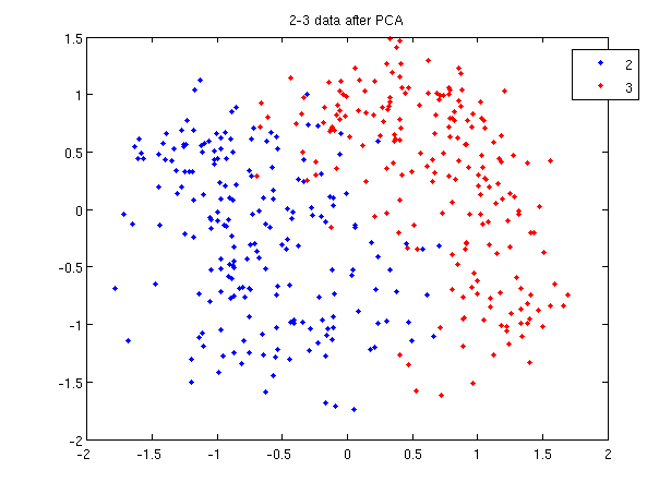
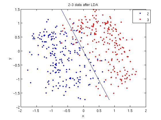
In class, we were shown an example of using LDA and QDA on the 2_3 data that is used in the first assignment. The code below reproduces that example, slightly modified, and explains each step.
>> load 2_3;
>> [U, sample] = princomp(X');
>> sample = sample(:,1:2);
- First, we do principal component analysis (PCA) on the 2_3 data to reduce the dimensionality of the original data from 64 dimensions to 2. Doing this makes it much easier to visualize the results of the LDA and QDA algorithms.
>> plot (sample(1:200,1), sample(1:200,2), '.');
>> hold on;
>> plot (sample(201:400,1), sample(201:400,2), 'r.');
- Recall that in the 2_3 data, the first 200 elements are images of the number two handwritten and the last 200 elements are images of the number three handwritten. This code sets up a plot of the data such that the points that represent a 2 are blue, while the points that represent a 3 are red.
title and legend for information on adding the title and legend.- Before using
classifywe can set up a vector that contains the actual labels for our data, to train the classification algorithm. If we don't know the labels for the data, then the element in thegroupvector should be an empty string orNaN. (See grouping data for more information.)
>> group = ones(400,1);
>> group(201:400) = 2;
- We can now classify our data.
>> [class, error, POSTERIOR, logp, coeff] = classify(sample, sample, group, 'linear');
- The full details of this line can be examined in the Matlab help file linked above. What we care about are
class, which contains the labels that the algorithm thinks that each data point belongs to, andcoeff, which contains information about the line that algorithm created to separate the data into each class.
- We can see the efficacy of the algorithm by comparing
classtogroup.
>> sum (class==group)
ans =
   369
- This compares the value in
classto the value ingroup. The answer of 369 tells us that the algorithm correctly determined the class of the point 369 times, out of a possible 400 data points. This gives us an empirical error rate of 0.0775.
- We can see the line produced by LDA using
coeff.
>> k = coeff(1,2).const;
>> l = coeff(1,2).linear;
>> f = sprintf('0 = %g+%g*x+%g*y', k, l(1), l(2));
>> ezplot(f, [min(sample(:,1)), max(sample(:,1)), min(sample(:,2)), max(sample(:,2))]);
- Those familiar with the programming language C will find the
sprintfline refreshingly familiar; those with no exposure to C are directed to Matlab'ssprintfpage. Essentially, this code sets up the equation of the line in the form0 = a + bx + cy. We then use theezplotfunction to plot the line.
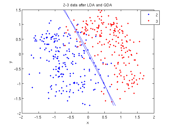
- Let's perform the same steps, except this time using QDA. The main difference with QDA is a slightly different call to
classify, and a more complicated procedure to plot the line.
>> [class, error, POSTERIOR, logp, coeff] = classify(sample, sample, group, 'quadratic');
>> sum (class==group)
ans =
   371
>> k = coeff(1,2).const;
>> l = coeff(1,2).linear;
>> q = coeff(1,2).quadratic;
>> f = sprintf('0 = %g+%g*x+%g*y+%g*x^2+%g*x.*y+%g*y.^2', k, l, q(1,1), q(1,2)+q(2,1), q(2,2));
>> ezplot(f, [min(sample(:,1)), max(sample(:,1)), min(sample(:,2)), max(sample(:,2))]);
classify can also be used with other discriminant analysis algorithms. The steps laid out above would only need to be modified slightly for those algorithms.
Recall: An analysis of the function of princomp in matlab.
In our assignment 1, we have learnt that how to perform Principal Component Analysis using SVD method. In fact, the matlab offers us a function called princomp which can perform PCA conveniently. From the matlab help file on princomp, you can find the details about this function. But here we will analyze the code of the function of princomp() in matlab to find something different when comparing with SVD method. The following is the code of princomp and explanations to some emphasized steps.
   function [pc, score, latent, tsquare] = princomp(x);
   %   PRINCOMP Principal Component Analysis (centered and scaled data).
   %   [PC, SCORE, LATENT, TSQUARE] = PRINCOMP(X) takes a data matrix X and
   %   returns the principal components in PC, the so-called Z-scores in SC
   %   ORES, the eigenvalues of the covariance matrix of X in LATENT,
   %   and Hotelling's T-squared statistic for each data point in TSQUARE.
   %   Reference: J. Edward Jackson, A User's Guide to Principal Components
   %   John Wiley & Sons, Inc. 1991 pp. 1-25.
   %   B. Jones 3-17-94
   %   Copyright 1993-2002 The MathWorks, Inc.
   %   $Revision: 2.9 $  $Date: 2002/01/17 21:31:45 $
   [m,n] = size(x);       %  get the lengh of the rows and columns of matrix x.
   r = min(m-1,n);        %  max possible rank of X
   avg = mean(x);         %  the mean of every column of X
   centerx = (x - avg(ones(m,1),:));
                          %  centers X by subtracting off column means
   [U,latent,pc] = svd(centerx./sqrt(m-1),0);
                          %  "economy size" decomposition
   score = centerx*pc;
                          %  the representation of X in the principal component space
   if nargout < 3
      return;
    end
    latent = diag(latent).^2;
    if (r   latent = [latent(1:r); zeros(n-r,1)];
    score(:,r+1:end) = 0;
    end
    if nargout < 4
    return;
    end
    tmp = sqrt(diag(1./latent(1:r)))*score(:,1:r)';
    tsquare = sum(tmp.*tmp)';
From the above code, we should pay attention to the following aspects when comparing with SVD method:
First, Rows of [math]\displaystyle{ \,X }[/math] correspond to observations, columns to variables. When using princomp on 2_3 data in assignment 1, note that we take the transpose of [math]\displaystyle{ \,X }[/math].
 >> load 2_3;
 >> [U, score] = princomp(X');
Second, princomp centers X by subtracting off column means.
The third, when [math]\displaystyle{ \,X=UdV' }[/math], princomp uses [math]\displaystyle{ \,V }[/math] as coefficients for principal components, rather than [math]\displaystyle{ \,U }[/math].
The following is an example to perform PCA using princomp and SVD respectively to get the same results.
- SVD method
 >> load 2_3
 >> mn=mean(X,2);
 >> X1=X-repmat(mn,1,400);
 >> [s d v]=svd(X1');
 >> y=X1'*v;
- princomp
>>[U score]=princomp(X');
Then we can see that y=score, v=U.
useful resouces: LDA and QDA in Matlab[3],[4],[5]
Reference
The Elements of Statistical Learning: Data Mining, Inference, and Prediction
The Elements of Statistical Learning: Data Mining, Inference, and Prediction, Second Edition, February 2009 Trevor Hastie, Robert Tibshirani, Jerome Friedman
http://www-stat.stanford.edu/~tibs/ElemStatLearn/ (3rd Edition is available)
