CatBoost: unbiased boosting with categorical features: Difference between revisions
No edit summary |
No edit summary |
||
| Line 34: | Line 34: | ||
In ordered boosting, the algorithm starts with generating <math>s+1</math> independent random permutations <math>\sigma_0, \sigma_1, \dots, \sigma_s</math> of the training dataset. <math>\sigma_1, \dots, \sigma_s</math> contributes to the internal nodes of a tree where the evaluation of the splits takes place. <math>\sigma_0</math> contributes to the terminal nodes where the leaf value is determined. the algorithm starts with building a decision tree based on the base predictors. The same splitting criterion is used in building a decision tree in the context of ordered boosting. Note that the trees built under this model are symmetric as this helps to improvise the algorithm in terms of its runtime. | In ordered boosting, the algorithm starts with generating <math>s+1</math> independent random permutations <math>\sigma_0, \sigma_1, \dots, \sigma_s</math> of the training dataset. <math>\sigma_1, \dots, \sigma_s</math> contributes to the internal nodes of a tree where the evaluation of the splits takes place. <math>\sigma_0</math> contributes to the terminal nodes where the leaf value is determined. the algorithm starts with building a decision tree based on the base predictors. The same splitting criterion is used in building a decision tree in the context of ordered boosting. Note that the trees built under this model are symmetric as this helps to improvise the algorithm in terms of its runtime. | ||
Define <math>M_{r,j}(i)</math> as our current model for the ''i''-th sample based on the first ''j'' samples. A random permutation <math>\sigma_r</math> is sampled from the <math>s+1</math> independent random permutations of the training dataset. A gradient is computed at each step such that <math>grad_{r,j}(i)=\frac{\delta{L(y_i,M_{r,j}(i))}}{\delta{s}}</math>. The leaf value for the tree constructed based on the ''i''-th sample will then be equals to the average of the gradients computed. When a tree, <math>T_t</math> is constructed, the tree itself is used to boost all the existing models <math>M_{r',j}</math>. Finally, in our final model, <math>F</math>, the leaf values are computed using the standard gradient boosting procedure. See Figure 2 for the detailed algorithm of how CatBoost build a decision tree. | Define <math>M_{r,j}(i)</math> as our current model for the ''i''-th sample based on the first ''j'' samples. A random permutation <math>\sigma_r</math> is sampled from the <math>s+1</math> independent random permutations of the training dataset. The random permutation, says <math>\sigma_r</math>, will then contribute to our construction of tree, <math>T_t</math> at each iteration. | ||
A gradient is computed at each step such that <math>grad_{r,j}(i)=\frac{\delta{L(y_i,M_{r,j}(i))}}{\delta{s}}</math>. The leaf value for the tree constructed based on the ''i''-th sample will then be equals to the average of the gradients computed, which can be written as: | |||
$$avg grad_{r, \sigma_r(i)-1}$$. When a tree, <math>T_t</math> is constructed, the tree itself is used to boost all the existing models <math>M_{r',j}</math>. Finally, in our final model, <math>F</math>, the leaf values are computed using the standard gradient boosting procedure. See Figure 2 for the detailed algorithm of how CatBoost build a decision tree. | |||
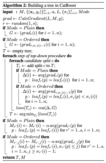
[[File:Catboost tree algorithm.png | center]] | [[File:Catboost tree algorithm.png | center]] | ||
<div align="center">Figure 2: Algorithm to build a tree in Catboost</div> | <div align="center">Figure 2: Algorithm to build a tree in Catboost</div> | ||
Revision as of 17:10, 18 November 2021
Presented by
Jessie Man Wai Chin, Yi Lin Ooi, Yaqi Shi, Shwen Lyng Ngew
Introduction
This paper presents a deep convolutional neural network architecture codenamed Inception. This newly designed architecture enhances the utilization of the computing resources by increasing the depth and width of the network, while maintaining the computational budget constraint. DNNs are powerful because they can perform arbitrary parallel computation for a modest number of steps. The proposed architecture was implemented through a 22 layers deep network called GoogLeNet and significantly outperformed the state of the art in the ImageNet Large-Scale Visual Recognition Challenge 2014 (ILSVRC14).
Previous Work
The current architecture is built on the network-in-network approach proposed by Lin et al.[1] for the purpose of increase the representation power of the neural networks. They added additional 1 X 1 convolutional layers, serving as dimension reduction modules to significantly reduce the number of parameters of the model. The paper also took inspiration from the Regions with Convolutional Neural Networks (R-CNN) proposed by Girshick et al. [2]. The overall detection problem is divided into two subproblems:
1. Utilize low-level cues for potential object proposals
2. Classify object categories with CNN
Motivation
Gradient boosting is known to be a popular and powerful machine learning method that could potentially increase the accuracy of a model. It aims to identify strong predictors in a model by performing gradient descent. Nevertheless, there exists a statistical issue which makes gradient boosting less powerful as we intended it to be. The paper identified this issue as prediction shift caused by target leakage.
A prediction shift happens when there is a shift between the predicted model trained on the training samples and the distribution of the test samples. This often occurs as the predicted model is trained using all training samples and not all training samples are fully representative of the test samples. When the predicted model is trained using all training samples, it could lead to a biased model since the model has seen the labels during its learning stage. In gradient boosting, the current estimate [math]\displaystyle{ F^t }[/math] is based on the previous model [math]\displaystyle{ F^{t-1} }[/math] we built on earlier in each iteration. To better demonstrate a prediction shift, it essentially means that [math]\displaystyle{ F^{t-1}(\bf{x_k})|\bf{x_k} }[/math] where [math]\displaystyle{ \bf{x_k} }[/math] comes from training samples is shifted from [math]\displaystyle{ F^{t-1}(\bf{x})|\bf{x} }[/math] where [math]\displaystyle{ \bf{x} }[/math] comes from testing samples. This is caused by target leakage where the distribution of the estimated model is different from the distribution of the testing samples. Therefore, the model is biased and could lead to overfitting in some cases. To identify this issue, we will introduce ordered boosting which is the motivation behind categorical boosting.
Ordered Target Statistics
Before the introduction of ordered boosting, we will first introduce the concept of ordered target statistics. The reason why ordered target statistics is used in this algorithm is to avoid overfitting. In ordered target statistics, a random permutation on the training samples is constructed so that we train our model based on the new training samples in which our current model has never seen previously. Define a target statistic as [math]\displaystyle{ \hat{x}_k^i = E(y | x^i = x_k^i) }[/math] where [math]\displaystyle{ k }[/math] refers to [math]\displaystyle{ k^{th} }[/math] training samples and [math]\displaystyle{ i }[/math] refers to [math]\displaystyle{ i^{th} }[/math] categorical feature.
In ordered target statistics, a random permutation [math]\displaystyle{ \sigma }[/math] is generated to help the algorithm to obtain training samples sequentially. For instance, if we would like to obtain [math]\displaystyle{ k^{th} }[/math] training samples, then [math]\displaystyle{ D_k = {x_j : \sigma(j)\lt \sigma(k)} }[/math]. Through this method, we can ensure that the model is unbiased as the trained model is obtained based on the new samples in which the model has never seen. In the traditional boosting method, the model is obtained based on all the training samples which could possibly lead to overfitting as we train the model based on what the model has seen previously. Therefore, the issue of overfitting motivates the idea of ordered target statistics which we will use to generate the permutations of our training samples.
Ordered Boosting
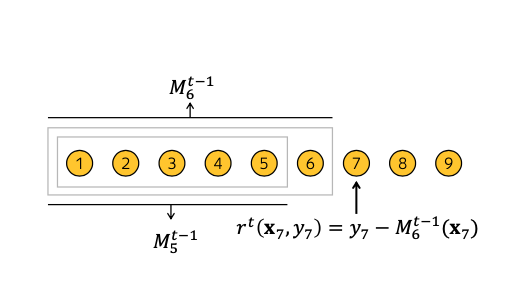
To overcome the prediction shift discussed in the previous section, ordered boosting is introduced. In ordered boosting, a new training dataset is obtained in each step of boosting. This means that the model is trained such that the model we obtained previously is applied to this set of new training samples. This guarantees that the model in which we have obtained previously has not seen the labels in the new training set. Therefore, the trained model at each step of boosting is not biased. To better illustrate this, assuming [math]\displaystyle{ M_t }[/math] is our current model in [math]\displaystyle{ {t+1}^{th} }[/math] iteration which is learned using only the first t samples, the residual [math]\displaystyle{ r^{t+1} = y_i - M_{t} }[/math] is unshifted since the model is trained without the observations in the new training set. This is supported by the generation of random permutations [math]\displaystyle{ \sigma }[/math] of our training samples. To illustrate this idea, please see Figure (1).

In ordered boosting, the algorithm starts with generating [math]\displaystyle{ s+1 }[/math] independent random permutations [math]\displaystyle{ \sigma_0, \sigma_1, \dots, \sigma_s }[/math] of the training dataset. [math]\displaystyle{ \sigma_1, \dots, \sigma_s }[/math] contributes to the internal nodes of a tree where the evaluation of the splits takes place. [math]\displaystyle{ \sigma_0 }[/math] contributes to the terminal nodes where the leaf value is determined. the algorithm starts with building a decision tree based on the base predictors. The same splitting criterion is used in building a decision tree in the context of ordered boosting. Note that the trees built under this model are symmetric as this helps to improvise the algorithm in terms of its runtime.
Define [math]\displaystyle{ M_{r,j}(i) }[/math] as our current model for the i-th sample based on the first j samples. A random permutation [math]\displaystyle{ \sigma_r }[/math] is sampled from the [math]\displaystyle{ s+1 }[/math] independent random permutations of the training dataset. The random permutation, says [math]\displaystyle{ \sigma_r }[/math], will then contribute to our construction of tree, [math]\displaystyle{ T_t }[/math] at each iteration.
A gradient is computed at each step such that [math]\displaystyle{ grad_{r,j}(i)=\frac{\delta{L(y_i,M_{r,j}(i))}}{\delta{s}} }[/math]. The leaf value for the tree constructed based on the i-th sample will then be equals to the average of the gradients computed, which can be written as: $$avg grad_{r, \sigma_r(i)-1}$$. When a tree, [math]\displaystyle{ T_t }[/math] is constructed, the tree itself is used to boost all the existing models [math]\displaystyle{ M_{r',j} }[/math]. Finally, in our final model, [math]\displaystyle{ F }[/math], the leaf values are computed using the standard gradient boosting procedure. See Figure 2 for the detailed algorithm of how CatBoost build a decision tree.

ILSVRC 2014 Challenge Results
The proposed architecture was implemented through a deep network called GoogLeNet as a submission for ILSVRC14’s Classification Challenge and Detection Challenge.
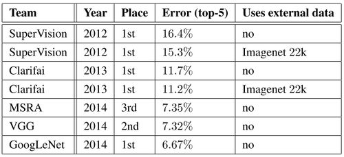
The classification challenge is to classify images into one of 1000 categories in the Imagenet hierarchy. The top-5 error rate - the percentage of test examples for which the correct class is not in the top 5 predicted classes - is used for measuring accuracy. The results of the classification challenge is shown in Table 1. The final submission of GoogLeNet obtains a top-5 error of 6.67% on both the validation and testing data, ranking first among all participants, significantly outperforming top teams in previous years, and not utilizing external data.

The ILSVRC detection challenge asks to produce bounding boxes around objects in images among 200 classes. Detected objects count as correct if they match the class of the groundtruth and their bounding boxes overlap by at least 50%. Each image may contain multiple objects (with different scales) or none. The mean average precision (mAP) is used to report performance. The results of the detection challenge is listed in Table 2. Using the Inception model as a region classifier, combining Selective Search and using an ensemble of 6 CNNs, GoogLeNet gave top detection results, almost doubling accuracy of the the 2013 top model.

Conclusion
Googlenet outperformed the other previous deep learning networks, and it became a proof of concept that approximating the expected optimal sparse structure by readily available dense building blocks (or the inception modules) is a viable method for improving the neural networks in computer vision. The significant quality gain is at a modest increase for the computational requirement is the main advantage for this method. Even without performing any bounding box operations to detect objects, this architecture gained a significant amount of quality with a modest amount of computational resources.
Critiques
By using nearly 5 million parameters, GoogLeNet, compared to previous architectures like VGGNet and AlexNet, reduced the number of parameters in the network by almost 92%. This enabled Inception to be used for many big data applications where a huge amount of data was needed to be processed at a reasonable cost while the computational capacity was limited. However, the Inception network is still complex and susceptible to scaling. If the network is scaled up, large parts of the computational gains can be lost immediately. Also, there was no clear description about the various factors that lead to the design decision of this inception architecture, making it harder to adapt to other applications while maintaining the same computational efficiency.
-
References
[1] L. Bottou and Y. L. Cun. Large scale online learning. In Advances in neural information processing systems, pages 217–224, 2004.
[2] L. Breiman. Out-of-bag estimation, 1996.
[3] L. Breiman. Using iterated bagging to debias regressions. Machine Learning, 45(3):261–277, 2001.
[4] L. Breiman, J. Friedman, C. J. Stone, and R. A. Olshen. Classification and regression trees. CRC press, 1984.
[5] R. Caruana and A. Niculescu-Mizil. An empirical comparison of supervised learning algorithms. In Proceedings of the 23rd international conference on Machine learning, pages 161–168. ACM, 2006.
[6] B. Cestnik et al. Estimating probabilities: a crucial task in machine learning. In ECAI, volume 90, pages 147–149, 1990.
[7] O. Chapelle, E. Manavoglu, and R. Rosales. Simple and scalable response prediction for display advertising. ACM Transactions on Intelligent Systems and Technology (TIST), 5(4):61, 2015.
[8] T. Chen and C. Guestrin. Xgboost: A scalable tree boosting system. In Proceedings of the 22Nd ACM SIGKDD International Conference on Knowledge Discovery and Data Mining, pages 785–794. ACM, 2016.
[9] M. Ferov and M. Modr `y. Enhancing lambdamart using oblivious trees. arXiv preprint arXiv:1609.05610, 2016.
[10] J. Friedman, T. Hastie, and R. Tibshirani. Additive logistic regression: a statistical view of boosting. The annals of statistics, 28(2):337–407, 2000.
[11] J. Friedman, T. Hastie, and R. Tibshirani. The elements of statistical learning, volume 1. Springer series in statistics New York, 2001.
[12] J. H. Friedman. Greedy function approximation: a gradient boosting machine. Annals of statistics, pages 1189–1232, 2001.
[13] J. H. Friedman. Stochastic gradient boosting. Computational Statistics & Data Analysis, 38(4):367–378, 2002.
[14] A. Gulin, I. Kuralenok, and D. Pavlov. Winning the transfer learning track of yahoo!’s learning to rank challenge with yetirank. In Yahoo! Learning to Rank Challenge, pages 63–76, 2011.
[15] X. He, J. Pan, O. Jin, T. Xu, B. Liu, T. Xu, Y. Shi, A. Atallah, R. Herbrich, S. Bowers, et al. Practical lessons from predicting clicks on ads at facebook. In Proceedings of the Eighth International Workshop on Data Mining for Online Advertising, pages 1–9. ACM, 2014.
[16] G. Ke, Q. Meng, T. Finley, T. Wang, W. Chen, W. Ma, Q. Ye, and T.-Y. Liu. Lightgbm: A highly efficient gradient boosting decision tree. In Advances in Neural Information Processing Systems, pages 3149–3157, 2017.
[17] M. Kearns and L. Valiant. Cryptographic limitations on learning boolean formulae and finite automata. Journal of the ACM (JACM), 41(1):67–95, 1994.
[18] J. Langford, L. Li, and T. Zhang. Sparse online learning via truncated gradient. Journal of Machine Learning Research, 10(Mar):777–801, 2009. 10
[19] LightGBM. Categorical feature support. http://lightgbm.readthedocs.io/en/latest/Advanced-Topics.html#categorical-feature-support, 2017.
[20] LightGBM. Optimal split for categorical features. http://lightgbm.readthedocs.io/en/latest/Features.html#optimal-split-for-categorical-features, 2017.
[21] LightGBM. feature_histogram.cpp. https://github.com/Microsoft/LightGBM/blob/master/src/treelearner/feature_histogram.hpp, 2018.
[22] X. Ling, W. Deng, C. Gu, H. Zhou, C. Li, and F. Sun. Model ensemble for click prediction in bing search ads. In Proceedings of the 26th International Conference on World Wide Web Companion, pages 689–698. International World Wide Web Conferences Steering Committee, 2017.
[23] Y. Lou and M. Obukhov. Bdt: Gradient boosted decision tables for high accuracy and scoring efficiency. In Proceedings of the 23rd ACM SIGKDD International Conference on Knowledge Discovery and Data Mining, pages 1893–1901. ACM, 2017.
[24] L. Mason, J. Baxter, P. L. Bartlett, and M. R. Frean. Boosting algorithms as gradient descent. In Advances in neural information processing systems, pages 512–518, 2000.
[25] D. Micci-Barreca. A preprocessing scheme for high-cardinality categorical attributes in classifi-cation and prediction problems. ACM SIGKDD Explorations Newsletter, 3(1):27–32, 2001.
[26] B. P. Roe, H.-J. Yang, J. Zhu, Y. Liu, I. Stancu, and G. McGregor. Boosted decision trees as an alternative to artificial neural networks for particle identification. Nuclear Instruments and Methods in Physics Research Section A: Accelerators, Spectrometers, Detectors and Associated Equipment, 543(2):577–584, 2005.
[27] L. Rokach and O. Maimon. Top–down induction of decision trees classifiers — a survey. IEEE Transactions on Systems, Man, and Cybernetics, Part C (Applications and Reviews), 35(4):476–487, 2005.
[28] D. B. Rubin. The bayesian bootstrap. The annals of statistics, pages 130–134, 1981.
[29] Q. Wu, C. J. Burges, K. M. Svore, and J. Gao. Adapting boosting for information retrieval measures. Information Retrieval, 13(3):254–270, 2010.
[30] K. Zhang, B. Schölkopf, K. Muandet, and Z. Wang. Domain adaptation under target and conditional shift. In International Conference on Machine Learning, pages 819–827, 2013.
[31] O. Zhang. Winning data science competitions. https://www.slideshare.net/ShangxuanZhang/winning-data-science-competitions-presented-by-owen-zhang,2015.
[32] Y. Zhang and A. Haghani. A gradient boosting method to improve travel time prediction. Transportation Research Part C: Emerging Technologies, 58:308–324, 2015.