markov Random Fields for Super-Resolution: Difference between revisions
No edit summary |
No edit summary |
||
| Line 20: | Line 20: | ||
<center><math> | <center><math> | ||
\hat{x}_{jMMSE} = \sum_{x_j} \sum_{all x_i, i != j} P(x_1,x_2,...,x_N,y_1,y_2,...,y_N) | \hat{x}_{jMMSE} = \sum_{x_j} \sum_{all x_i, i != j} P(x_1,x_2,...,x_N,y_1,y_2,...,y_N) | ||
</math> | </math> (2)</center> | ||
<center><math> | <center><math> | ||
\hat{x}_{jMAP} = \arg\max_{x_j} (max_{all x_i != j} P(x_1,x_2,...,x_N,y_1,y_2,...,y_N) | \hat{x}_{jMAP} = \arg\max_{x_j} (max_{all x_i != j} P(x_1,x_2,...,x_N,y_1,y_2,...,y_N)) | ||
</math></center> | </math> (3)</center> | ||
For large networks the computation of Eq(2) and Eq(3) are infeasible to evaluate directly; however, the task is easier for network which are trees or chains. | For large networks the computation of Eq(2) and Eq(3) are infeasible to evaluate directly; however, the task is easier for network which are trees or chains. | ||
| Line 32: | Line 32: | ||
<center><math>\begin{matrix} | <center><math>\begin{matrix} | ||
\hat{x}_{MAP} & = & \arg\max_{x_1} ( max_{x_2} max_{x_3} P(x_1,x_2,x_3,y_1,y_2,y_3 | \hat{x}_{MAP} & = & \arg\max_{x_1} ( max_{x_2} max_{x_3} P(x_1,x_2,x_3,y_1,y_2,y_3)\\ | ||
& = & \arg\max_{x_1} ( max_{x_2} max_{x_3} \phi(x_1,y_1) \phi(x_2,y_2) \phi(x_3,y_3) \psi(x_1,x_2) \psi(x2,x3)\\ | & = & \arg\max_{x_1} ( max_{x_2} max_{x_3} \phi(x_1,y_1) \phi(x_2,y_2) \phi(x_3,y_3) \psi(x_1,x_2) \psi(x2,x3)\\ | ||
& = & \arg\max_{x_1} \phi(x_1,y_1) (max_{x_2} \psi(x_1,x_2) \phi(x_2,y2)) (max_{x_3} \psi(x_2, x_3) \phi(x_3,y_3)\\ | & = & \arg\max_{x_1} \phi(x_1,y_1) (max_{x_2} \psi(x_1,x_2) \phi(x_2,y2)) (max_{x_3} \psi(x_2, x_3) \phi(x_3,y_3)\\ | ||
\end{matrix}</math></center> | \end{matrix}</math> (4)</center> | ||
The similar expressions for <math>x_{2MAP}</math> and <math>x_{3MAP}</math> can be used. Equations (3) and (2) can be computed by iterating the following steps. The MAP estimate at node j is | The similar expressions for <math>x_{2MAP}</math> and <math>x_{3MAP}</math> can be used. Equations (3) and (2) can be computed by iterating the following steps. The MAP estimate at node j is | ||
<center><math> | <center><math> | ||
\hat{x}_{jMAP} = \arg\max_{x_j} \phi(x_j, y_j) \prod_{k} M^k_j | \hat{x}_{jMAP} = \arg\max_{x_j} \phi(x_j, y_j) \prod_{k} M^k_j | ||
</math></center> | </math> (5)</center> | ||
Where k runs over all “scene” node neighbors of node j, and <math> M^k_j </math> is the message from node k to node j. The <math>M^k_j</math> message is calculated by: | Where k runs over all “scene” node neighbors of node j, and <math> M^k_j </math> is the message from node k to node j. The <math>M^k_j</math> message is calculated by: | ||
<center><math> | <center><math> | ||
M^k_j = max_{x_k} \psi(x_j,x_k) \phi(x_k,y_k) \prod_{i!=j} \hat{M}^l_k | M^k_j = max_{x_k} \psi(x_j,x_k) \phi(x_k,y_k) \prod_{i!=j} \hat{M}^l_k | ||
</math></center> | </math> (6)</center> | ||
where <math>\hat{M}^l_k</math> is <math>M^k_l</math> from the previous iteration. The initial <math>\hat{M}^k_j</math>'s are set to column vector of 1’s, with the same dimension as <math>x_j</math>. Because the initial messages are 1’s at the first iteration, all the message in the network are: | where <math>\hat{M}^l_k</math> is <math>M^k_l</math> from the previous iteration. The initial <math>\hat{M}^k_j</math>'s are set to column vector of 1’s, with the same dimension as <math>x_j</math>. Because the initial messages are 1’s at the first iteration, all the message in the network are: | ||
<center><math> | <center><math> | ||
M^2_1 = max_{x_2} \psi(x_1, x_2) \phi(x_2,y_2 | M^2_1 = max_{x_2} \psi(x_1, x_2) \phi(x_2,y_2) | ||
</math></center> | </math> (7)</center> | ||
<center><math> | <center><math> | ||
M^3_2 = max_{x_3} \psi(x_2, x_3) \phi(x_3,y_3 | M^3_2 = max_{x_3} \psi(x_2, x_3) \phi(x_3,y_3) | ||
</math></center> | </math> (8)</center> | ||
<center><math> | <center><math> | ||
M^1_2 = max_{x_1} \psi(x_2, x_1) \phi(x_1,y_1 | M^1_2 = max_{x_1} \psi(x_2, x_1) \phi(x_1,y_1) | ||
</math></center> | </math> (9)</center> | ||
<center><math> | <center><math> | ||
M^2_3 = max_{x_2} \psi(x_3, x_2) \phi(x_2,y_2 | M^2_3 = max_{x_2} \psi(x_3, x_2) \phi(x_2,y_2) | ||
</math></center> | </math> (10)</center> | ||
The second iteration uses the messages above as the <math>\hat{M}</math> variables in Eq(6) : | The second iteration uses the messages above as the <math>\hat{M}</math> variables in Eq(6) : | ||
<center><math> | <center><math> | ||
M^2_1 = max_{x_2} \psi(x_1, x_2) \phi(x_2,y_2)\hat{M}^3_2 | M^2_1 = max_{x_2} \psi(x_1, x_2) \phi(x_2,y_2)\hat{M}^3_2 | ||
</math></center> | </math> (11)</center> | ||
<center><math> | <center><math> | ||
M^3_2 = max_{x_3} \psi(x_2, x_3) \phi(x_3,y_3 | M^3_2 = max_{x_3} \psi(x_2, x_3) \phi(x_3,y_3) | ||
</math></center> | </math> (12)</center> | ||
<center><math> | <center><math> | ||
M^2_3 = max_{x_2} \psi(x_3, x_2) \phi(x_2,y_2)\hat{M}^1_2 | M^2_3 = max_{x_2} \psi(x_3, x_2) \phi(x_2,y_2)\hat{M}^1_2 | ||
</math></center> | </math> (13)</center> | ||
<center><math> | <center><math> | ||
M^1_2 = max_{x_1} \psi(x_2, x_1) \phi(x_1,y_1 | M^1_2 = max_{x_1} \psi(x_2, x_1) \phi(x_1,y_1) | ||
</math></center> | </math> (14)</center> | ||
And thus | And thus | ||
<center><math> | <center><math> | ||
M^2_1 = max_{x_2} \psi(x_1, x_2) \phi(x_2,y_2) * max_{x_3} \psi(x_2,x_3) \phi(x_3,y_3 | M^2_1 = max_{x_2} \psi(x_1, x_2) \phi(x_2,y_2) * max_{x_3} \psi(x_2,x_3) \phi(x_3,y_3) | ||
</math></center> | </math> (15)</center> | ||
Eventually the MAP estimates for <math>x_1</math> becomes: | Eventually the MAP estimates for <math>x_1</math> becomes: | ||
Revision as of 11:38, 13 November 2011
A Summary on
Markov Networks for Super-Resolution
by
W. T. Freeman and E. C. Pasztor
Introduction
There are some applications in computer vision in which the task is to infer the unobserved image called “scene” from the observed “image”. Typically, estimating the entire “scene” image at once is too complex and infeasible, and thus a common approach is to process the image regions locally and then generalize the interpretations across space. The interpretation of images can be done by modeling the relationship between local regions of “images” and “scenes”, and between neighboring local “scene” regions. The former allows us to estimate initial guess for “scene”, and the latter propagates the estimation. These problems are so-called low-level vision problems. Freeman first introduced a probabilistic approach <ref name="R1"> W. T. Freeman, E. C. Pasztor, and O. T. Carmichael, "Learning Low-Level Vision", International Journal of Computer Vision, 40(1), pp. 25-47, 2000.</ref> <ref name="R2"> W. Freeman and E. Pasztor, "Markov Networks for Super-Resolution", in Proc. of 34th Annual Conference on Information Sciences and Systems, Princeton University, March 2000.</ref> in which they try to exploit training method using “image”/ “scene” pairs and apply the Bayesian inference of graphical models. The method is called VISTA, Vision by Image/Scene TrAining. The authors have shown the advantages of the proposed model in different practical applications. Here we focus on super-resolution application where the problem is to estimate high resolution details from low resolution images.
Markov Networks for low-level vision problems
A common graphical model for low-level vision problems is Markov networks. For a given "image", [math]\displaystyle{ y }[/math], the underlying "scene" [math]\displaystyle{ x }[/math] should be estimated. The posterior probability, [math]\displaystyle{ P(x|y)= cP(x,y) }[/math] is calculated considering the fact that the parameter [math]\displaystyle{ c = 1/P(y) }[/math] is a constant over [math]\displaystyle{ x }[/math]. The best scene estimate [math]\displaystyle{ \hat{x} }[/math] is the minimum mean squared error, MMSE, or the maximum a posterior, MAP. Without any approximation the [math]\displaystyle{ \hat{x} }[/math] is difficult to compute. Therefore the "image" and "scene" are divided into patches and one node of the Markov network is assigned to each patch. Figure
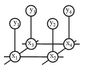
depicts the undirected graphical model for mentioned problem where the nodes connected by lines indicate statistical dependencies. Each “scene” node is connected to its corresponding “image” node as well as its neighbors.
To make use of Markov networks the unknown parameters should be learned from training data in learning phase, and then in inference phase the “scene” estimation can be made. For a Markov random field, the joint probability over the “scene” [math]\displaystyle{ x }[/math] and the “image” [math]\displaystyle{ y }[/math] is given by:
where [math]\displaystyle{ \psi }[/math] and [math]\displaystyle{ \phi }[/math] are potential functions and they are leaned from training data. In this paper the authors prefer to call these functions compatibility functions. Then one can write the MAP and the MMSE estimates for <math\hat{x}_j</math> by marginalizing or taking the maximum over all other variables in the posterior probability, respectively. For discrete variables the expression is:
For large networks the computation of Eq(2) and Eq(3) are infeasible to evaluate directly; however, the task is easier for network which are trees or chains.
Inference in Networks without loops
For networks with no loop the inference is the simple “message-passing” rule which enables us to compute MAP and MMSE estimate <ref name="R3"> Jordan, M.I. (Ed.). 1998. Learning in Graphical Models. MIT Press: Cambridge, MA </ref>. For example for the network in Figure 2
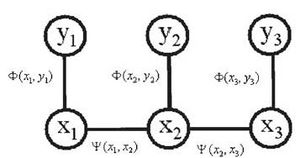
the MAP estimation for node [math]\displaystyle{ j }[/math] is determined by:
The similar expressions for [math]\displaystyle{ x_{2MAP} }[/math] and [math]\displaystyle{ x_{3MAP} }[/math] can be used. Equations (3) and (2) can be computed by iterating the following steps. The MAP estimate at node j is
Where k runs over all “scene” node neighbors of node j, and [math]\displaystyle{ M^k_j }[/math] is the message from node k to node j. The [math]\displaystyle{ M^k_j }[/math] message is calculated by:
where [math]\displaystyle{ \hat{M}^l_k }[/math] is [math]\displaystyle{ M^k_l }[/math] from the previous iteration. The initial [math]\displaystyle{ \hat{M}^k_j }[/math]'s are set to column vector of 1’s, with the same dimension as [math]\displaystyle{ x_j }[/math]. Because the initial messages are 1’s at the first iteration, all the message in the network are:
The second iteration uses the messages above as the [math]\displaystyle{ \hat{M} }[/math] variables in Eq(6) :
And thus
Eventually the MAP estimates for [math]\displaystyle{ x_1 }[/math] becomes:
The MMSE estimate Eq(3) has analogous formulate with the [math]\displaystyle{ max_{x_k} }[/math] of Eq(8) replaced by [math]\displaystyle{ \sum_{x_k} }[/math] and [math]\displaystyle{ \arg\max_{x_j} }[/math] replaced by [math]\displaystyle{ \sum_{x_j} x_j }[/math].
Networks with loops
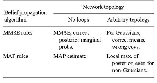
Although the belief propagation algorithm is derived for the networks without loops, Weiss and Freeman demonstrate the propagation rules works even in the network with loops <ref name="R4"> Weiss, Y. and Freeman, W.T. 1999. Correctness of belief propagation
in Gaussian graphical models of arbitrary topology. Technical Report UCB.CSD-99-1046, Berkeley. </ref> Summary of results from Weiss and Freeman regarding belief propagation results after convergence is provided in Figure 3. Fig.3
General view of the paper
Basically this paper aims to develop a new super-resolution scheme utilizing Markov random fields by which given low resolution image is resized to required high resolution size reproducing high frequency details. Typical interpolation techniques such as bilinear, nearest neighbor and bicubic expand the size of the low-resolution image, yet the result suffers from blurriness and in some cases blocking artifact.
According to Freeman, in this method they collect many pairs of high resolution images and their corresponding low-resolution images as the training set. Given low-resolution image y a typical bicubic interpolation algorithm is employed to create a high resolution image which is interpreted as the “image” in Markov network. Of course this image does not look suitable, and thus they try to estimate original high resolution image which in we may call it “scene” image based on the definitions provided above. In order to do that, the images in training set and also the low-resolution image is divided into patches so that each patch represents the Markov network node (figure1). Therefore, [math]\displaystyle{ y_i }[/math]’s in figure are observed, and thus should be shaded. Subsequently, for each patch in y 10 or 20 nearest patches from the training database are selected using Euclidean distance. The ultimate job is to find the best patch in the candidate set for each patch in y using MAP estimate. In other words, the estimated scene at each patch is always some example from the training set.
Implementation of low-level vision problems using Markov network
The “image” and “scene” are arrays of pixel values, and so the complete representation is cumbersome. In this research, the principle component analysis (PCA) is applied for each patch to find a set of lower dimensional basis function. Moreover, potential functions [math]\displaystyle{ \psi }[/math] and [math]\displaystyle{ \phi }[/math] should be determined. A nice idea is to define Gaussian mixtures over joint spaces [math]\displaystyle{ x_i*x_j }[/math] and [math]\displaystyle{ x_j*x_k }[/math];however, it is very difficult. The authors prefer a discrete representation where the most straightforward approach is to evenly sample all possible states of each image and scene variable at each patch.
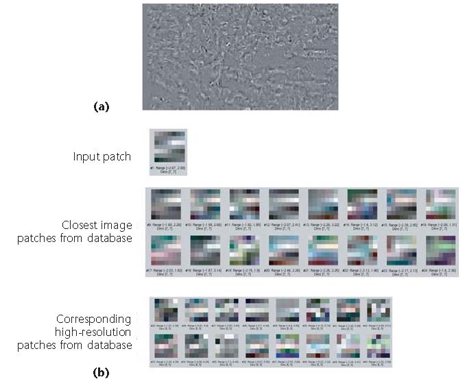
For each patch in "image" y a set of 10 or 20 "scene" candidates from the training set are chosen. Figure4
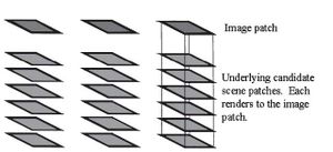
illustrates an example of each patch in y and the associated "scene" candidates.
Learning the Potential (Compatibility) Functions
The potential functions are defined arbitrary, but they have to be introduced wisely. In this paper, a simple way is used to find potential functions. They assume “scene” patches have overlap shown is Figure 5
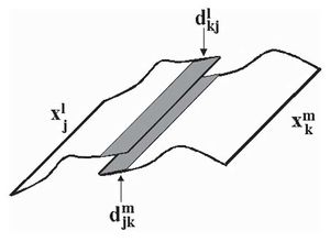
Therefore, the scene patches themselves may be use to define potential functions [math]\displaystyle{ \psi }[/math] between nodes [math]\displaystyle{ x_i }[/math]’s. Recall for node [math]\displaystyle{ x_i }[/math] and its neighbor [math]\displaystyle{ x_j }[/math] there are two sets of candidate patches. Let assume the lth candidate in node j and the mth candidate in node k have some overlap. Also, we can think that the pixels in the overlapped region in [math]\displaystyle{ x_j }[/math] ([math]\displaystyle{ d^l_{kj} }[/math]) and their correspondent in [math]\displaystyle{ x_k }[/math] ([math]\displaystyle{ d^m_{jk} }[/math]) are some variation of each other , and thus eventually the potential function between node [math]\displaystyle{ x_j }[/math] and node [math]\displaystyle{ x_k }[/math] are given by:
Where [math]\displaystyle{ \sigma_s }[/math] has to be determined. The authors assume that the image and scene training samples differ from the "ideal" or original high resolution image by Gaussian noise with covariance <math\sigma_i</math> and [math]\displaystyle{ \sigma_s }[/math], respectively. Therefore, [math]\displaystyle{ \psi }[/math] function between node j and k can be represented by a matrix whose lth row and mth column is [math]\displaystyle{ \psi(x^l_k, x^m_j) }[/math]. Potential function [math]\displaystyle{ \phi }[/math] which is defined between "scene" node x and "image" node y is determined based on another intuitive assumption. We say that a "scene" candidate [math]\displaystyle{ x^k_l }[/math] is compatible with an observed image patch [math]\displaystyle{ y_0 }[/math] if the image patch, [math]\displaystyle{ y^k_l }[/math], associated with the scene candidate [math]\displaystyle{ x^k_l }[/math] in the training database matches [math]\displaystyle{ y_0 }[/math]. Of course, it will not exactly match, but we may suppose that the training data is “noisy” version of original image resulting in:
Super-Resolution
For the super-resolution problem, the input is a low-resolution image, and the “scene” to be estimated is its high resolution version. At the first glance, the task may seem impossible since the high resolution data is missing. However, the human eye is able to identify edges and sharp details in low resolution image and we know these structural information should remain at higher resolution level. The authors attempt to solve this problem using aforementioned Markov model and they name the method VISTA. There are some preprocessing steps in order to increase the efficiency of the training set. First, consider three scales Laplacian pyramid decomposition. The first sub-band, H, represents the detail in high frequency while the second and the third sub-bands indicate the middle, M, and the low, L, frequency components. The assumption is that high frequency band, H, is conditionally independent of the lower frequency bands, given the middle frequency band, M, yielding:
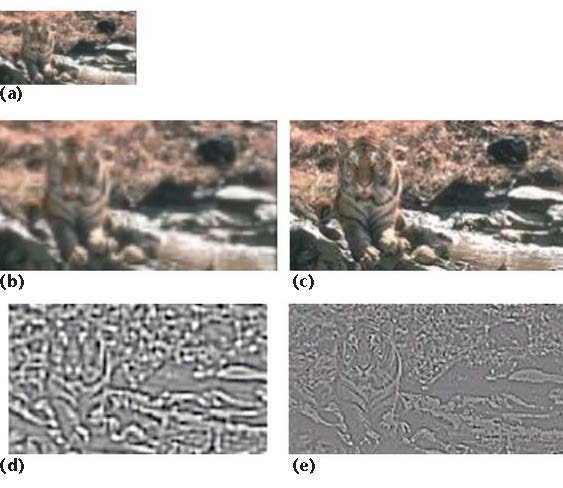
Hence, to predict the high frequency components, we will need the middle frequency details, M, not the low frequency band, L. This hypothesis greatly reduces the computation costs. Second, The reaserchers in this paper assume that statistical relationships between image bands are independent of image contrast. Furthermore, they take the absolute value of the mid-frequency band, and then pass it through a lowpass filter resulting in a normalized mid frequency band. They also do the same procedure for high-frequency band. Figure 5 (a) show the low-resolution image which then is expanded to have the same size as the desired high resolution image using a typical interpolation algorithms such as bicubic method (Figure 5 (b)). The image in (c) in the original high resolution image. Images in Figure 5 (d) and (e) are the first level of the Laplacian pyramid decomposition for "image" and “scene” images, respectively. In other words, the high frequency component in Figure 5 (e) should be estimated using frequency component in Figure 5(d).
Figure5
In order to utilize Markov network for this problem the "image" and "scene" images are divided into local patches as shown in Figure 6 and the final estimate for "scene" image , x,, is the collection which maximizes probability of [math]\displaystyle{ P(x|y) }[/math] using Equation 1.
Figure6
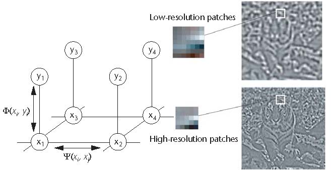
Figure 7 illustrates an example of a given patch in y and its corresponding "scene" patches. The patch size is a difficult task since choosing small size gives very little information for estimating the underlying “scene” patches. On the other hand, large patches would make the learning processs of [math]\displaystyle{ \phi }[/math]’s very complex. The authors in some papers use 7*7 patch size for low frequency band and 3*3 for high frequency components, but in ref they use 7*7 for the "image" and 5*5 for the "scene".
Figure7
Fugure 8 compares the results of the proposed approach in this paper and different super-resolution schemes. The interesting thing is the effect of training set on the final result. Because the estimate "scene" patch is always chosen from the training database the final result resembles the training set in some manner.
Figure8
References
<references />