Deep Residual Learning for Image Recognition Summary: Difference between revisions
No edit summary |
No edit summary |
||
| Line 1: | Line 1: | ||
== Presented by == | |||
Ethan Cyrenne, Dieu Hoa Nguyen, Mary Jane Sin, Carolyn Wang | |||
== Introduction == | == Introduction == | ||
Latest revision as of 12:01, 3 December 2021
Presented by
Ethan Cyrenne, Dieu Hoa Nguyen, Mary Jane Sin, Carolyn Wang
Introduction
Neural and convolutional neural networks have made significant progress in the field of classification. They consist of a number of layers each of which contain a number of nodes. The deeper the network, that is, the more layers a network has, the better it appears to be able to pick up on high level features in the data. However increasing the number of layers is difficult as it can result in issues with backpropagation, which is how the networks are trained. The 'vanishing gradient' problem has been addressed previously, and refers to instances where the gradient used in backpropagation becomes too small to make discernable differences as the parameters in the model are tuned, and thus the model is unable to evolve.
The purpose of residual learning is to solve the issue of degradation, which is the unexpected phenomenon where deeper networks have higher training and testing error than their shallower counterparts. In theory, this should not occur since the deeper network could be constructed as follows: assuming the shallower network has m layers, the first m layers of the deeper network are a copy of the shallower network, and the rest of the layers are identity layers whose output is the same as their input. This would result in the error values of the deeper network being at most equal to those of the shallower network. However, this result is not seen in practice.
Motivation
In general, classification problems aim to map the given data such that we may predict the class that it belongs to. The problem then becomes to approximate the underlying mapping of the problem. When networks gain depth, it becomes more difficult to train them as gradients may become very small. The authors developed a method that train a model to fit a residual mapping rather than directly fitting the underlying mapping. Thus, instead of fitting to the underlying mapping, the model is made to fit the underlying mapping plus the initial input [math]\displaystyle{ x }[/math].
It’s important to note that if the dimension of [math]\displaystyle{ x }[/math] is different from the output of a layer, we may use a linear mapping to convert it to the appropriate size. Furthermore, the method is computationally efficient and may be performed without calculating any extra parameters, so residual and normal models may still be compared meaningfully.
Model Architecture
After testing several plain and residual neural networks, the authors fitted the following models to the ImageNet dataset for comparison of accuracy:
Plain Network
This model is based on the VGG network and contains 34 weighted convolutional layers of mostly 3 × 3 filters. The number of filters in each layer is either the same or doubled, depending on whether the feature map size remains the same or halved. The network ends with a global average pooling layer and a 1000-way fully-connected layer with softmax. Compared to the VGG model, the plain network model has fewer filters and lower complexity.
Residual Network
The residual model is the plain model as proposed above with identity shortcuts added to each pair of 3 × 3 filters. These shortcut connections are directly added in the model when the input and output of the network have the same dimensions, otherwise a dimension mapping has to be performed first.
The ImageNet 2012 classification dataset was trained from scratch. Training data was pre-process by being resized with a 224 × 224 crop and subtracting the mean per-pixel value. Then, weights were initialized with batch normalization, and training started with a learning rate of 0.1, a weight decay of 0.0001, and a momentum of 0.9 and no dropout. In total, the models were trained for up to 60 × 104 iterations. Testing data was pre-processed with the standard 10-crop testing approach and passed into a fully-convolutional network to achieve comparison results.
ImageNet Classification
The authors used the ImageNet classification dataset to measure accuracy on different models.
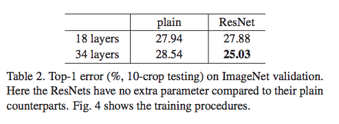
They first compare plain nets to ResNets with 18 and 34 layers. The ResNets are identical save for the identity shortcuts joining each two layer stack (A). Note that in order to change dimensions, they use zero-padded shortcuts. The 34-layer plain net gives a higher training error than its 18-layer counterpart (the degradation problem; shown above in Table 2). This discrepancy is attributed to exponentially low convergence rates since BN is used which should prevent vanishing gradients. The 34 layer ResNet performs better on the train set than its 18-layer counterpart and performs better than the 34-layer plain net. So, the degradation problem is addressed.
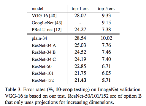
The authors also consider the use of projection shortcuts where: (B) projection shortcuts are only used for changing dimensions and (C) all shortcuts are projections. The use of projections improves accuracy since additional residual learning is added. However, this improvement is not practical when compared to the added time complexity.
To train deeper nets, they used the identity shortcut and modified the structure to a bottleneck design. The bottleneck design uses a stack of three layers instead of two in each residual function (shortcut) and cuts the time complexity in half. When applied to 50-layer, 101-layer, and 152-layer ResNets, accuracy improves (Table 3). The 152-layer model won 1st place in ILSVRC 2015.
CIFAR-10 and Analysis
Using the CIFAR-10 dataset, which consists of 50k training images and 10k testing images in 10 classes, the following shows the results of experiments trained on the training set and evaluated on the test set. The aim is to compare the behaviours of extremely deep networks using plain architectures and residual networks. A higher training error is observed when going deeper for deep plain nets. This phenomenon is similar to what was observed with the ImageNet dataset, suggesting that such an optimization difficulty is a fundamental problem. However, similar to the ImageNet case, the proposed architecture manages to overcome the optimization difficulty and reach accuracy gains as the depth increases. The training and testing errors are shown in the following graphs:
Reference
He, K., Zhang, X., Ren, S., & Sun, J. (2016). Deep residual learning for image recognition. In Proceedings of the IEEE conference on computer vision and pattern recognition (pp. 770-778).


