a neural representation of sketch drawings: Difference between revisions
No edit summary |
|||
| Line 124: | Line 124: | ||
== Critique == | == Critique == | ||
# The performance of the decoder model can hardly be evaluated. The authors present the performance of the decoder by showing the generated sketches, it is clear and straightforward, however, not very efficient. It would be great if the authors could present a way, or a metric to evaluate how well the sketches are generated rather than printing them out and evaluate with human judgement. | |||
# Same problem as the output, the authors didn't present an evaluation for the algorithms either. They provided ###Lr### and ###Lkl### for reference, however, a lower loss doesn't represent a better performance. | |||
# I understand that using strokes as inputs is a novel and innovative move, however, the paper does not provide a baseline or any comparison with other methods or algorithms. Some other researches were mentioned in the paper, using similar and smaller datasets. It would be great if the authors could use some basic or existing methods a baseline and compare with the new algorithm. | |||
# Besides the comparison with other algorithms, it would also be great if the authors could remove or replace some component of the algorithm in the model to show if one part is necessary, or what made them decide to include a specific component in the algorithm. | |||
# The authors proposed a few future applications for the model, however, the current output seems somehow not very close to their descriptions. But I do believe that this is a very good beginning, with the release of the sketch dataset, it must attract more scholars to research and improve with it! | |||
== References == | == References == | ||
Revision as of 00:05, 17 November 2018
Introduction
In this paper, The authors present a recurrent neural network: sketch-rnn to construct stroke-based drawings. Besides new robust training methods, they also outline a framework for conditional and unconditional sketch generation.
Neural networks have been heavily used as image generation tools, for example, Generative Adversarial Networks, Variational Inference and Autoregressive models. Most of those models are focusing on modelling pixels of the images. However, people learn to draw using sequences of strokes since very young ages. The authors decide to use this character to create a new model that utilize strokes of the images as a new approach to vector images generations and abstract concept generalization.
The model is trained with hand-drawn sketches as input sequences. The model is able to produce sketches in vector format. In the conditional generation model, they also explore the latent space representation for vector images and discuss a few future application of this model. The model and dataset are now available as an open source project.
Related Work
There are some works in the history that used a similar approach to generate images such as Portrait Drawing by Paul the Robot and some reinforcement learning approaches. They work more like a mimic of digitized photographs. There are some Neural network based approaches too, but those are mostly dealing with pixel images. Little work is done on vector images generation. There are models that use Hidden Markov Models or Mixture Density Networks to generate human sketches, continuous data points or vectorized Kanji characters.
The model also allows us to explore the latent space representation of vector images. There are previous works that achieved similar functions as well, such as combining Sequence-to-Sequence models with Variational Autoencoder to model sentences into latent space and using probabilistic program induction to model Omniglot dataset.
The dataset they use contains 50 million vector sketches. Before this paper, there is a Sketch data with 20k vector sketches, a Sketchy dataset with 70k vector sketches along with pixel images, and a ShadowDraw system that used 30k raster images along with extracted vectorized features. They are all comparatively small.
Methodology
Dataset
QuickDraw is a dataset with 50 million vector drawings collected by a game Quick Draw!. It contains hundreds of classes, each class has 70k training samples, 2.5k validation samples and 2.5k test samples.
The data format of each sample is a representation of a pen stroke action event. The Origin is the initial coordinate of the drawing. The sketches are points in a list. Each point consists of 5 elements ###( x, y, p 1 , p 2 , p 3 )### where x and y are the offset distance in x and y directions from the previous point. ### p1, p2 and p3### are three possible states in binary one-hot representation where ### p1 ### indicates the pen is touching the paper, ### p2 ### indicates the pen will be lifted from here, and ###p3### represents the drawing has ended.
Sketch-RNN
- image###
The model is a Sequence-to-Sequence Variational Autoencoder(VAE). The encoder is a bidirectional RNN, the input is a sketch sequence and a reversed sketch sequence, so there will be two final hidden states. The output is a size ###N_z### latent vector.
- eq1 ###
Then the authors project h into to ###mu and sigma###, convert ###mu### into non-negative and use them with ###N(0,I)### to construct a random vector ###z###.
- eq2###
Note that ###z### is not deterministic but a conditioned random vector.
The decoder is an autoregressive RNN. The initial hidden states are generated using ### [ h 0 ; c 0 ] = tanh(W z z + b z ) ###. ###s_0### is ###(0,0,1,0,0)### For each step i in the decoder, the input ###x_i### is the concatenation of previous point ###S_i-1### and latent vector z. The output are probability distribution parameters for the next data point ###S_i###. The authors model ###(deltax, delta y)### as a Gaussian mixture model (GMM) with M normal distributions and model ###(p1 p2 p3)### as categorical distribution where they sum up to 1. The generated sequence is conditioned from the latent vector ###z### that sampled from the encoder, which is end-to-end trained together with the decoder.
- eq3###
Here the ###N(x,y| .....)### i the probability distribution function for ###x,y###, ###ro_xy### is the correlation parameter for this bivariate normal distribution. The ### ### is a lenth M categorical distribution vector are the mixture weights of the Gaussian mixture model.
The output vector ###y_i### is generated using a fully-connected forward propagation in the hidden state of the RNN.
- eq4###
The output consists the probability distribution of the next data point.
- eq5###
- exp### and ###tanh### operations will be applied to standard deviations to ensure they are non-negative and between -1 and 1.
- eq6###
Categorical distribution probabilities for ###(p1,p2,p3)### using ###(q1,q2,q3)### can be obtained as :
- eq7###
It is hard do decide when to stop drawing because ###(p1,p2,p3)### is very unbalanced. scholars in the past used different weights for each pen event probability, but the authors have a better idea. They define a hyperparameter representing the max length of the longest sketch in the training set ###N_max###, and set the ### Si to be (0, 0, 0, 0, 1) for i > Ns.#
The outcome sample ###S_i'### can be generated in each time step during sample process and fed as input for the next time step. The process will stop when ###p3 = 1### or ###i = N_max###. The output is not deterministic but conditioned random sequences. The level of randomness can be controlled using a temperature parameter ###tao###.
- eq8###
The ###tao### ranges from 0 to 1. When ###tao = 0### the output will be deterministic as the sample will consist on the on the peak of the probability density function.
- fig 3###
Unconditional Generation
The decoder RNN could work as a standalone autoregressive model. In this case, initial states are 0, the input ###xi### is only ###s_i-1 or s'_i-1###.
Training
The training process is the same as a Variational Autoencoder. The loss function is the sum of Reconstruction Loss ###L_R### and the Kullback-Leibler Divergence Loss ###L_KL###. The reconstruction loss ###L_r### can be obtained with generated parameters of pdf and training data ###s###. It is the sum of the ###Ls### and ###Lp###, which are the log loss of the offset ###(delta x, delta y)### and the pen state ###(p1p2p3)###.
- eq 9###
Both terms are normalized by ###N_max###.
- L_kl### measures the difference between the distribution of the latent vector ###z### and an IID Gaussian vector with zero mean and unit variance.
- eq 10###
The overall loss is weighted as:
- eq 11###
When ###w_kl### = 0, the model becomes a standalone unconditional generator.
Experiments
The authors experiment with the sketch-rnn model using different settings and recorded both losses. They used a Long Short-Term Memory(LSTM) model as an encoder and a HyperLSTM as a decoder. They also conduct multi-class datasets. The result is as follows.
- tabel 1###
We could see the trade-off between ###Lr### and ###Lkl### in this table clearly.
Conditional Reconstruction
The authors assess the reconstructed sketch with a given sketch with different ###tao### values. We could see that with high ###tao### value on the right, the reconstructed sketches are more random.
- fig 5###
They also experiment on inputting a sketch from a different class. The output will still keep some features from the class that the model is trained on.
Latent Space Interpolation
The authors visualize the reconstruction sketches while interpolating between latent vectors using different ###wKL### values. With high ###wkl### values, the generated images are more coherently interpolated.
- fig 6###
Sketch Drawing Analogies
Since the latent vector ###z### encode conceptual features of a sketch, those features can also be used to augment other sketches that do not have these features. This is possible when models are trained with low ###Lkl### values. The authors are able to perform vector arithmetic on latent vectors from different sketches and explore how the model generates sketches base on these latent spaces.
Predicting Different Endings of Incomplete Sketches
This model is able to predict an incomplete sketch by encoding the sketch into hidden state ###h### using the decoder and then using ###h### as an initial hidden state to generate the remaining sketch.
- fig 7###
Applications and Future Work
The authors believe this model can assist artists by suggesting how to finish a sketch, helping them to find interesting intersections between different drawings or objects, or generating a lot of similar but different designs.
This model may also find its place on teaching students how to draw. When the model is trained with a high ###wkl### and sampled with a low ###tao###, it may help to turn a poor sketch into a more aesthetical sketch. Latent vector augmentation could also help to create a better drawing by inputting user-rating data during training processes.
It exciting that they manage to combine this model with other unsupervised, cross-domain pixel image generation models to create photorealistic images from sketches.
Conclusion
This paper introduced an interesting model sketch-rnn that can encode and decode sketches, generate and complete sketches. The authors demonstrated how to interpolate between latent spaces from different class and how to use it to augment sketches. They also showed that it's important to enforce a prior distribution on latent vector while interpolating coherent sketch generations.
Critique
- The performance of the decoder model can hardly be evaluated. The authors present the performance of the decoder by showing the generated sketches, it is clear and straightforward, however, not very efficient. It would be great if the authors could present a way, or a metric to evaluate how well the sketches are generated rather than printing them out and evaluate with human judgement.
- Same problem as the output, the authors didn't present an evaluation for the algorithms either. They provided ###Lr### and ###Lkl### for reference, however, a lower loss doesn't represent a better performance.
- I understand that using strokes as inputs is a novel and innovative move, however, the paper does not provide a baseline or any comparison with other methods or algorithms. Some other researches were mentioned in the paper, using similar and smaller datasets. It would be great if the authors could use some basic or existing methods a baseline and compare with the new algorithm.
- Besides the comparison with other algorithms, it would also be great if the authors could remove or replace some component of the algorithm in the model to show if one part is necessary, or what made them decide to include a specific component in the algorithm.
- The authors proposed a few future applications for the model, however, the current output seems somehow not very close to their descriptions. But I do believe that this is a very good beginning, with the release of the sketch dataset, it must attract more scholars to research and improve with it!
References
- Bahdanau, Dzmitry, Kyunghyun Cho, and Yoshua Bengio. "Neural machine translation by jointly learning to align and translate." arXiv preprint arXiv:1409.0473 (2014).
fonts and examples
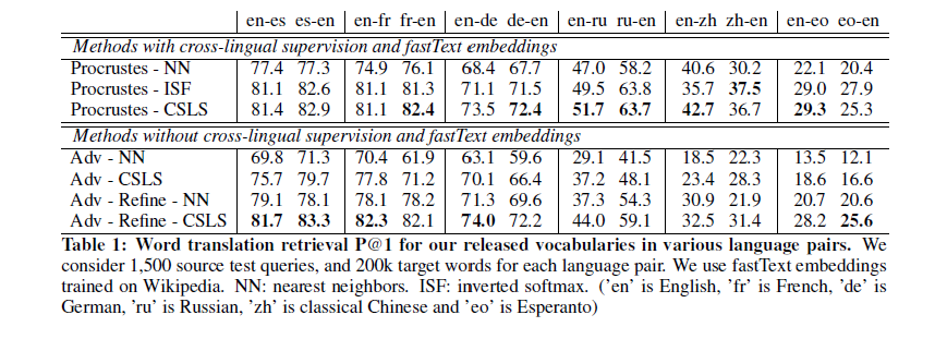
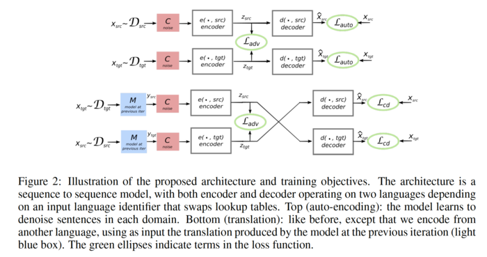
The unsupervised translation scheme has the following outline:
- The word-vector embeddings of the source and target languages are aligned in an unsupervised manner.
- Sentences from the source and target language are mapped to a common latent vector space by an encoder, and then mapped to probability distributions over
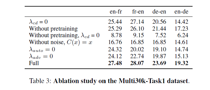
The objective function is the sum of:
- The de-noising auto-encoder loss,
I shall describe these in the following sections.


