One-Shot Imitation Learning

Introduction

Robotic systems can be used for many applications, but to truly be useful for complex applications, they need to overcome 2 challenges: having the intent of the task at hand communicated to them, and being able to perform the manipulations necessary to complete this task. It is preferable to use demonstration to teach the robotic systems rather than natural language, as natural language may often fail to convey the details and intricacies required for the task. However, current work on learning from demonstrations is only successful with large amounts of feature engineering or a large number of demonstrations. The proposed model aims to achieve 'one-shot' imitation learning, ie. learning to complete a new task from just a single demonstration of it without any other supervision. As input, the proposed model takes the observation of the current instance of a task, and a demonstration of successfully solving a different instance of the same task. Strong generalization was achieved by using a soft attention mechanism on both the sequence of actions and states that the demonstration consists of, as well as on the vector of element locations within the environment. The success of this proposed model at completing a series of block stacking tasks can be viewed at http://bit.ly/nips2017-oneshot.

Related Work

While one-shot imitation learning is a novel combination of ideas, each of the components has previously been studied.

• Imitation Learning:
  • Behavioural learning uses supervised learning to map from observations to actions (e.g. (Pomerleau 1988), (Ross et. al 2011))
  • Inverse reinforcement learning estimates a reward function that considers demonstrations as optimal behavior (e.g. (Ng et. al 2000))
• One-Shot Learning:
  • Typically a form of meta-learning
  • Previously used for variety of tasks but all domain-specific
  • (Finn et al. 2017) proposed a generic solution but excluded imitation learning
• Reinforcement Learning:
  • Demonstrated to work on variety of tasks and environments, in particular on games and robotic control
  • Requires large amount of trials and a user-specified reward function
• Multi-task/Transfer Learning:
  • Shown to be particularly effective at computer vision tasks
  • Not meant for one-shot learning
• Attention Modelling:
  • The proposed model makes use of the attention model from (Bahdanau et al. 2016)
  • The attention modelling over demonstration is similar in nature to the seq2seq models from the well known (Sutskever et al. 2014)

One-Shot Imitation Learning

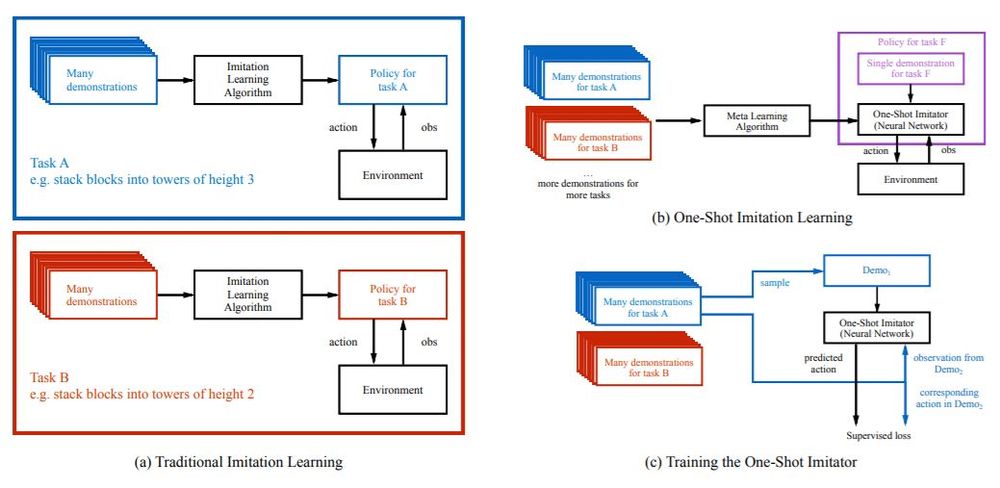
The figure above shows the differences between traditional and one-shot imitation learning. In a), the traditional method may require training different policies for performing similar tasks that are similar in nature. For example, stacking blocks to a height of 2 and to a height of 3. In b), the one-shot imitation learning allows the same policy to be used for these tasks given a single demonstration, achieving good performance without any additional system interactions. In c), the policy is trained by using a set of different training tasks, with enough examples so that the learned results can be generalized to other similar tasks. Each task has a set of successful demonstrations. Each iteration of training uses two demonstrations from a task, one is used as the input passing into the algorithm and the other is used at the output, the results from the two are then conditioned to produce the correct action.

Problem Formalization

The problem is briefly formalized with the authors describing a distribution of tasks, an individual task, a distribution of demonstrations for this task, and a single demonstration respectively as \[T, \: t\sim T, \: D(t), \: d\sim D(t)\] In addition, an action, an observation, parameters, and a policy are respectively defined as \[a, o, \theta, \pi_\theta(a|o,d)\] In particular, a demonstration is a sequence of observation and action pairs \[d = [(o_1, a_1),(o_2, a_2), . . . ,(o_H , a_H )]\] Assuming that [math]\displaystyle{ H }[/math], the length or horizon of a demonstration, and some evaluation function $$R_t(d): R^T \rightarrow R$$ are given, and that succesful demonstrations are available for each task, then the objective is to maximize expectation of the policy performance over \[t\sim T, d\sim D(t)\].

Block Stacking Tasks

The tasks that the authors focus on is block stacking. A user specifies in what final configuration cubic blocks should be stacked, and the goal is to use a 7-DOF Fetch robotic arm to arrange the blocks in this configuration. The number of blocks, and their desired configuration (ie. number of towers, the height of each tower, and order of blocks within each tower) can be varied and encoded as a string. For example, 'abc def' would signify 2 towers of height 3, with block A on block B on block C in one tower, and block D on block E on block F in a second tower. To add complexity, the initial configuration of the blocks can vary and is encoded as a set of 3-dimensional vectors describing the position of each block relative to the robotic arm.

Algorithm

To avoid needing to specify a reward function, the authors use behavioral cloning and DAGGER, 2 imitation learning methods that require only demonstrations, for training. In each training step, a list of tasks is sampled, and for each, a demonstration with injected noise along with some observation-action pairs are sampled. Given the current observation and demonstration as input, the policy is trained against the sampled actions by minimizing L2 norm for continuous actions, and cross-entropy for discrete ones. Adamax is used as the optimizer with a learning rate of 0.001.

Architecture

The authors propose a novel architecture for imitation learning, consisting of 3 networks.

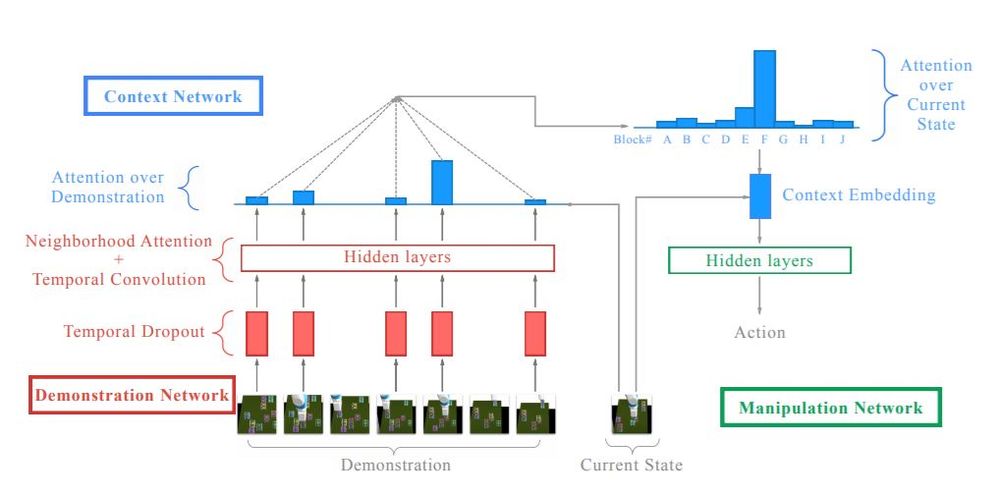
While, in principle, a generic neural network could learn the mapping from demonstration and current observation to appropriate action, the authors propose the following architecture which they claim as one of the main contributions of this paper, and believe it would be useful for complex tasks in the future. The proposed architecture consists of three modules: the demonstration network, the context network, and the manipulation network.

Demonstration Network

This network takes a demonstration as input and produces an embedding with size linearly proportional to the number of blocks and the size of the demonstration.

Temporal Dropout

Since a demonstration for block stacking can be very long, the authors randomly discard 95% of the time steps, a process they call 'temporal dropout'. The reduced size of the demonstrations allows multiple trajectories to be explored during testing to calculate an ensemble estimate. Dilated temporal convolutions and neighborhood attention are then repeatedly applied to the downsampled demonstrations.

Neighborhood Attention

Since demonstration sizes can vary, a mechanism is needed that is not restricted to fixed-length inputs. While soft attention is one such mechanism, the problem with it is that there may be increasingly large amounts of information lost if soft attention is used to map longer demonstrations to the same fixed length as shorter demonstrations. As a solution, the authors propose having the same number of outputs as inputs, but with attention performed on other inputs relative to the current input.

A query [math]\displaystyle{ q }[/math], a list of context vectors [math]\displaystyle{ \{c_j\} }[/math], and a list of memory vectors [math]\displaystyle{ \{m_j\} }[/math] are given as input to soft attention. Each attention weight is given by the product of a learned weight vector and a nonlinearity applied to the sum of the query and corresponding context vector. Softmaxed weights applied to the corresponding memory vector form the output of the soft attention.

\[Inputs: q, \{c_j\}, \{m_j\}\] \[Weights: w_i \leftarrow v^Ttanh(q+c_i)\] \[Output: \sum_i{m_i\frac{\exp(w_i)}{\sum_j{\exp(w_j)}}}\]

A list of same-length embeddings, coming from a previous neighbourhood attention layer or a projection from the list of block coordinates, is given as input to neighborhood attention. For each block, two separate linear layers produce a query vector and a context vector, while a memory vector is a list of tuples that describe the position of each block joined with the input embedding for that block. Soft attention is then performed on this query, context vector, and memory vector. The authors claim that the intuition behind this process is to allow each block to provide information about itself relative to the other blocks in the environment. Finally, for each block, a linear transformation is performed on the vector composed by concatenating the input embedding, the result of the soft attention for that block, and the robot's state.

For an environment with B blocks: \[State: s\] \[Block_i: b_i \leftarrow (x_i, y_i, z_i)\] \[Embeddings: h_1^{in}, ..., h_B^{in}\] \[Query_i: q_i \leftarrow Linear(h_i^{in})\] \[Context_i: c_i \leftarrow Linear(h_i^{in})\] \[Memory_i: m_i \leftarrow (b_i, h_i^{in}) \] \[Result_i: result_i \leftarrow SoftAttn(q_i, \{c_j\}_{j=1}^B, \{m_k\}_{k=1}^B)\] \[Output_i: output_i \leftarrow Linear(concat(h_i^{in}, result_i, b_i, s))\]

Context network

This network takes the current state and the embedding produced by the demonstration network as inputs and outputs a fixed-length "context embedding" which captures only the information relevant for the manipulation network at this particular step.

Attention over demonstration

The current state is used to compute a query vector which is then used for attending over all the steps of the embedding. Since at each time step there are multiple blocks, the weights for each are summed together to produce a scalar for each time step. Neighbourhood attention is then applied several times, using an LSTM with untied weights, since the information at each time steps needs to be propagated to each block's embedding.

Performing attention over the demonstration yields a vector whose size is independent of the demonstration size; however, it is still dependent on the number of blocks in the environment, so it is natural to now attend over the state in order to get a fixed-length vector.

Attention over current state

The authors propose that in general, within each subtask, only a limited number of blocks are relevant for performing the subtask. If the subtask is to stack A on B, then intuitively, one would suppose that only block A and B are relevant, and perhaps any blocks that may be blocking access to either A or B. This is not enforced during training, but once soft attention is applied to the current state to produce a fixed-length context embedding, the authors believe that the model does indeed learn in this way.

Manipulation network

Given the context embedding as input, this simple feedforward network decides on the particular action needed, to complete the subtask of stacking one particular 'source' block on top of another 'target' block.

Experiments

The proposed model was tested on the block stacking tasks. the experiments were designed at answering the following questions:

• How does training with behavioral cloning compare with DAGGER?
• How does conditioning on the entire demonstration compare to conditioning on the final state?
• How does conditioning on the entire demonstration compare to conditioning on a “snapshot” of the trajectory?
• Can the authors' framework generalize to tasks that it has never seen during training?

For the experiments, 140 training tasks and 43 testing tasks were collected, each with between 2 to 10 blocks and a different, desired final layout. Over 1000 demonstrations for each task were collected using a hard-coded policy rather than a human user. The authors compare 4 different architectures in these experiments:

• Behavioural cloning used to train the proposed model
• DAGGER used to train the proposed model
• The proposed model, trained with DAGGER, but conditioned on the desired final state rather than an entire demonstration
• The proposed model, trained with DAGGER, but conditioned on a 'snapshot' of the environment at the end of each subtask (ie. every time a block is stacked on another block)

Performance Evaluation

The most confident action at each timestep is chosen in 100 different task configurations, and results are averaged over tasks that had the same number of blocks. The results suggest that the performance of each of the architectures is comparable to that of the hard-coded policy which they aim to imitate. Performance degrades similarly across all architectures and the hard-coded policy as the number of blocks increases. On the harder tasks, conditioning on the entire demonstration led to better performance than conditioning on snapshots or on the final state. The authors believe that this may be due to the lack of information when conditioning only on the final state as well as due to regularization caused by temporal dropout which leads to data augmentation when conditioning on the full demonstration but is omitted when conditioning only on the snapshots or final state. Both DAGGER and behavioral cloning performed comparably well. As mentioned above, noise injection was used in training to improve performance; in practice, additional noise can still be injected but some may already come from other sources.

Visualization

The authors visualize the attention mechanisms underlying the main policy architecture to have a better understanding about how it operates. There are two kinds of attention that the authors are mainly interested in, one where the policy attends to different time steps in the demonstration, and the other where the policy attends to different blocks in the current state. The figures below show some of the policy attention heatmaps over time.

Conclusions

The proposed model successfully learns to complete new instances of a new task from just a single demonstration. The model was demonstrated to work on a series of block stacking tasks. The authors propose several extensions including enabling few-shot learning when one demonstration is insufficient, using image data as the demonstrations, and attempting many other tasks aside from block stacking.

Criticisms

While the paper shows an incredibly impressive result: the ability to learn a new task from just a single demonstration, there are a few points that need clearing up. Firstly, the authors use a hard-coded policy in their experiments rather than a human. It is clear that the performance of this policy begins to degrade quickly as the complexity of the task increases. It would be useful to know what this hard-coded policy actually was, and if the proposed model could still have comparable performance if a more successful demonstration, perhaps one by a human user, were performed. Give the current popularity of adversarial examples, it would also be interesting to see the performance when conditioned on an "adversarial" demonstration, that achieves the correct final state, but intentionally performs complex or obfuscated steps to get there. Second, it would be useful to see the model's performance on a more complex family of tasks than block stacking, since although each block stacking task is slightly different, the differences may turn out be insignificant compared to other tasks that this model should work on if it is to be a general imitation learning architecture; intuitively, the space of all possible moves and configurations is not large for the task. Also it is a bit misleading as there seems to be a need for more demonstrations to first get a reasonable policy that can generalize, leading to generic policy and then use just one demonstration on a new task expecting the policy to generalize. So it seems there is some sort of pre training involved here. Regardless, this work is a big step forward for imitation learning, permitting a wider range of tasks for which there is little training data and no reward function available, to still be successfully solved.

Illustrative Example: Particle Reaching

Figure 1: [Left] Agent, [Middle] Orange square is target, [Right] Green triangle is target [2].

Another simple yet insightful example of the One-Shot Imitation Learning is the particle reaching problem which provides a relatively simple suite of tasks from which the network needs to solve an arbitrary one. The problem is formulated such that for each task: there is an agent which can move based on a 2D force vector, and n landmarks at varying 2D locations (n varies from task to task) with the goal of moving the agent to the specific landmark reached in the demonstration. This is illustrated in Figure 1.

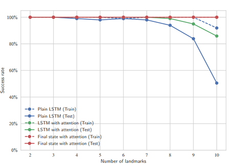
Figure 2: Experimental results [2].

Some insight comes from the use of different network architectures to solve this problem. The three architectures to compare (described below) are plain LSTM, LSTM with attention, and final state with attention. The key insight is that the architectures go from generic to specific, with the best generalization performance achieved with the most specific architecture, final state with attention, as seen in Figure 2. It is important to note that this conclusion does not carry forward to more complicated tasks such as the block stacking task.

• Plain LSTM: 512 hidden units, with the input being the demonstration trajectory (the position of the agent changes over time and approaches one of the targets). Output of the LSTM with the current state (from the task needed to be solved) is the input for a multi-layer perceptron (MLP) for finding the solution.
• LSTM with attention: Output of LSTM is now a set of weights for the different targets during training. These weights and the test state are used in the test task. The, now, 2D output is the input for an MLP as before.
• Final state with attention: Looks only at the final state of the demonstration since it can sufficiently provide the needed detail of which target to reach (trajectory is not required). Similar to previous architecture, produces weights used by MLP.

Source

1. Bahdanau, Dzmitry, Kyunghyun Cho, and Yoshua Bengio. "Neural machine translation by jointly learning to align and translate." arXiv preprint arXiv:1409.0473 (2014).
2. Duan, Yan, Marcin Andrychowicz, Bradly Stadie, OpenAI Jonathan Ho, Jonas Schneider, Ilya Sutskever, Pieter Abbeel, and Wojciech Zaremba. "One-shot imitation learning." In Advances in neural information processing systems, pp. 1087-1098. 2017.
3. Y. Duan, M. Andrychowicz, B. Stadie, J. Ho, J. Schneider, I. Sutskever, P. Abbeel, and W. Zaremba. One-shot imitation learning. arXiv preprint arXiv:1703.07326, 2017. (Newer revision)
4. Finn, Chelsea, Pieter Abbeel, and Sergey Levine. "Model-agnostic meta-learning for fast adaptation of deep networks." arXiv preprint arXiv:1703.03400 (2017).
5. Sutskever, Ilya, Oriol Vinyals, and Quoc V. Le. "Sequence to sequence learning with neural networks." Advances in neural information processing systems. 2014.