User:T358wang: Difference between revisions
| (15 intermediate revisions by 7 users not shown) | |||
| Line 5: | Line 5: | ||
== Introduction == | == Introduction == | ||
Landmark recognition is an image retrieval task with its | Landmark recognition is an image retrieval task with unique applications which comes with its own specific challenges. It can be used in robotics to localize robots for navigation and also used by manipulators to detect different objects. This paper provides a new and effective method to recognize landmark images which can successfully identify statues, buildings, and other different characteristic objects. A relatable use-case is auto-sorting collections of photos to determine the location of the landmark, something we see occur in our smartphone's photo albums. | ||
There are many difficulties encountered in the development process: | There are many difficulties encountered in the development process: | ||
| Line 11: | Line 11: | ||
'''1.''' The concept of landmarks is not strictly defined. Landmarks can take various forms including objects and buildings. | '''1.''' The concept of landmarks is not strictly defined. Landmarks can take various forms including objects and buildings. | ||
'''2.''' The same landmark can be photographed from different angles. Certain angles may capture the interior of a building as opposed to its exterior. This could result in vastly different picture characteristics between angles. A good model should accurately identify landmarks regardless of | '''2.''' The same landmark can be photographed from different angles. Certain angles may capture the interior of a building as opposed to its exterior. This could result in vastly different picture characteristics between angles. A good model should accurately identify landmarks regardless of angles viewed. | ||
'''3.''' Often landmarks photographed at different times of the day | '''3.''' Often landmarks photographed at different times of the day look different based on the lighting and/or shift in shadows that the model needs to consider. | ||
'''4.''' The dataset is unbalanced. The majority of objects fall into the single class of "not landmarks", while relatively few images exist for each class of landmark. Hence, it | '''4.''' The dataset is unbalanced. The majority of objects fall into the single class of "not landmarks", while relatively few images exist for each class of landmark. Hence, it is challenging to obtain both a low false-positive rate and a high recognition accuracy between classes of landmarks. | ||
There are also three potential problems: | There are also three potential problems: | ||
'''1.''' The processed data set contains a little error content | '''1.''' The processed data set contains a little error content; the image content is not clean, and the quantity is huge. | ||
'''2.''' The algorithm | '''2.''' The algorithm to learn the training set must be fast and scalable. | ||
'''3.''' While displaying high-quality judgment landmarks, there is no image geographic information mixed. | '''3.''' While displaying high-quality judgment landmarks, there is no image geographic information mixed. | ||
The article describes the deep convolutional neural network (CNN) architecture, loss function, training method, and inference aspects. Using this model, similar metrics to the state of the art model in the test were obtained and the inference time was found to be 15 times faster. | The article describes the deep convolutional neural network (CNN) architecture, loss function, training method, and inference aspects. Using this model, similar metrics to the state of the art model in the test were obtained and the inference time was found to be 15 times faster. Furthermore, because of the efficient architecture, the system can be implemented in an online system. The results of quantitative experiments are displayed through testing and deployment effect analysis to prove the effectiveness of the model. | ||
== Related Work == | == Related Work == | ||
| Line 32: | Line 32: | ||
Vector of Locally Aggregated Descriptors which uses first-order statistics of the local descriptor is one of the main representatives of local features-based methods. Another method is to selectively match the kernel Hamming embedding method extension. With the advent of deep convolutional neural networks, the most effective image retrieval method is based on training CNNs for specific tasks. Deep networks are very powerful for semantic feature representation, which allows us to effectively use them for landmark recognition. This method shows good results but brings additional memory and complexity costs. | Vector of Locally Aggregated Descriptors which uses first-order statistics of the local descriptor is one of the main representatives of local features-based methods. Another method is to selectively match the kernel Hamming embedding method extension. With the advent of deep convolutional neural networks, the most effective image retrieval method is based on training CNNs for specific tasks. Deep networks are very powerful for semantic feature representation, which allows us to effectively use them for landmark recognition. This method shows good results but brings additional memory and complexity costs. | ||
The DELF (DEep local feature) by Noh et al. proved promising results. This method combines the classic local feature method with deep learning. This allows us to extract local features from the input image and then use RANSAC for geometric verification. Random Sample Consensus (RANSAC) is a method to smooth data containing a significant percentage of errors, which is ideally suited for applications in automated image analysis where interpretation is based on the data generated by error-prone feature detectors. The goal of the project is to describe a method for accurate and fast large-scale landmark recognition using the advantages of deep convolutional neural networks. | |||
The DELF (DEep local feature) by Noh et al. proved promising results. This method combines the classic local feature method with deep learning. The dense features are extracted through fully convolutional network (FCN). To handle changes of scale, an image pyramid is constructed, and FCN is applied. Features are localized based on the receptive fields. | |||
[[File:delf.png | thumb | center | 1000px | The network architectures used for training (Noh et al., 2016)]] | |||
This allows us to extract local features from the input image and then use RANSAC for geometric verification. Random Sample Consensus (RANSAC) is a method to smooth data containing a significant percentage of errors, which is ideally suited for applications in automated image analysis where interpretation is based on the data generated by error-prone feature detectors. The goal of the project is to describe a method for accurate and fast large-scale landmark recognition using the advantages of deep convolutional neural networks. | |||
== Methodology == | == Methodology == | ||
| Line 40: | Line 45: | ||
[[File:t358wang_landmark_recog_system.png |center|800px]] | [[File:t358wang_landmark_recog_system.png |center|800px]] | ||
The landmark CNN consists of three parts: the main network, the embedding layer and the classification layer. To obtain a CNN main network suitable for training landmark recognition model, fine-tuning is applied and several pre-trained backbones (Residual Networks) based on other similar datasets, including ResNet-50, ResNet-200, SE-ResNext-101 and Wide Residual Network (WRN-50-2), are evaluated based on inference quality and efficiency, displayed in the table below. Based on the evaluation results, WRN-50-2 is selected as the optimal backbone architecture. Fine-tuning is a very efficient technique in various computer vision applications because we can take advantage of everything the model has already learned and applied it to our specific task. | The landmark CNN consists of three parts: the main network, the embedding layer and the classification layer. To obtain a CNN main network suitable for training landmark recognition model, fine-tuning is applied and several pre-trained backbones (Residual Networks) based on other similar datasets, including ResNet-50, ResNet-200, SE-ResNext-101 and Wide Residual Network (WRN-50-2), are evaluated based on inference quality and efficiency, displayed in the table below. Residual networks are shallower architectures compared to usual deep networks and have their layers fit residuals mappings, <math> \mathcal{F}(x):= \mathcal{H}(x)-x </math>. The residual mappings are then recast into <math>\mathcal{F}(x)+x</math>. This is realized using shortcut connections to skip various layers and having the outputs added to the outputs of the stacked layers (He, Zhang, Ren, & Sun, 2016). Based on the evaluation results, WRN-50-2 is selected as the optimal backbone architecture. Fine-tuning is a very efficient technique in various computer vision applications because we can take advantage of everything the model has already learned and applied it to our specific task. | ||
[[File:t358wang_backbones.png |center|600px]] | [[File:t358wang_backbones.png |center|600px]] | ||
For the embedding layer, as shown in the below figure, the last fully-connected layer after the averaging pool is removed. Instead, a fully-connected 2048 <math>\times</math> 512 layer and a batch normalization | For the embedding layer, as shown in the below figure, the last fully-connected layer after the averaging pool is removed. Instead, a fully-connected 2048 <math>\times</math> 512 layer and a batch normalization layer is added as the embedding layer. After the batch normalization, a fully-connected 512 <math>\times</math> n layer is added as the classification layer. The below figure shows the overview of the CNN architecture of the landmark recognition system. | ||
[[File:t358wang_network_arch.png |center|800px]] | [[File:t358wang_network_arch.png |center|800px]] | ||
| Line 68: | Line 73: | ||
[[File:t358wang_algorithm2.png |center|600px]] | [[File:t358wang_algorithm2.png |center|600px]] | ||
We will now look at how the landmark database was created. The collection process was structured by countries, cities and landmarks. They divided the world into several regions: Europe, America, Middle East, Africa, Far East, Australia and Oceania. Within each region, cities were selected that contained a lot of significant landmarks, and some natural landmarks were filtered out as they are difficult to distinguish. Once the cities and landmarks were selected, both images and metadata were collected for each landmark. | We will now look at how the landmark database was created. The collection process was structured by countries, cities and landmarks. They divided the world into several regions: Europe, America, Middle East, Africa, Far East, Australia and Oceania. Within each region, cities were selected that contained a lot of significant landmarks, and some natural landmarks were filtered out as they are difficult to distinguish. These include landmarks such as parks and beaches, unless they're very notable and popular, for example Santa Monica Pier. Natural landmarks Once the cities and landmarks were selected, both images and metadata were collected for each landmark. | ||
[[File:landmarkcleaning.png | center | 400px]] | [[File:landmarkcleaning.png | center | 400px]] | ||
| Line 116: | Line 121: | ||
== Conclusion == | == Conclusion == | ||
In this paper, we were hoping to solve some difficulties that emerge when trying to apply landmark recognition with a scalable approach to the production level, which is the kind of implementation that has been deployed to production at scale and used for recognition of user photos in the Mail.ru cloud application: there might not be a clean & sufficiently large database for interesting tasks, algorithms should be fast, scalable, and should aim for low FP and high accuracy. | In this paper, we were hoping to solve some difficulties that emerge when trying to apply landmark recognition with a scalable approach to the production level, which is the kind of implementation that has been deployed to production at scale and used for recognition of user photos in the Mail.ru cloud application: there might not be a clean & sufficiently large database for interesting tasks, algorithms should be fast, scalable, and should aim for low FP and high accuracy. The basis of this method is the use of embedded deep convolutional neural networks. The CNN is trained through course learning techniques and has a modified version of the center loss. To determine whether there are a landmark image embedding vector and one or more centroids of each class on the given image. | ||
While aiming for these goals, we presented a way of cleaning landmark data. And most importantly, we introduced the usage of embeddings of deep CNN to make recognition fast and scalable, trained by curriculum learning techniques with modified versions of Center loss. Compared to the state-of-the-art methods, this approach shows similar results but is much faster and suitable for implementation on a large scale. | While aiming for these goals, we presented a way of cleaning landmark data. And most importantly, we introduced the usage of embeddings of deep CNN to make recognition fast and scalable, trained by curriculum learning techniques with modified versions of Center loss. Compared to the state-of-the-art methods, this approach shows similar results but is much faster and suitable for implementation on a large scale. | ||
| Line 152: | Line 157: | ||
It would be better that if the summary have an extended usage of the model. For instance, if this model can applied to any other aspects rather than landmark recognition. It will give us a more general understanding of the model. | It would be better that if the summary have an extended usage of the model. For instance, if this model can applied to any other aspects rather than landmark recognition. It will give us a more general understanding of the model. | ||
It is really important that all the data comes from one format, such as all comes from an image. Because sometimes it is really expensive to go scan the land structure in person, and the form of images is more common. So it is better that the author can focus on one form so that cleaner data can be captured. | |||
In the introduction, it was claimed that the deep CNN could be used in an online fashion due to its efficiency. It would be better if the author could provide a benchmark of existing methods and the model given in this paper in an online fashion to compare their accuracy and efficiency. | |||
== References == | == References == | ||
| Line 159: | Line 168: | ||
2018. Revisiting Oxford and Paris: Large-Scale Image Retrieval Benchmarking. | 2018. Revisiting Oxford and Paris: Large-Scale Image Retrieval Benchmarking. | ||
arXiv preprint arXiv:1803.11285 (2018). | arXiv preprint arXiv:1803.11285 (2018). | ||
[3] He, K., Zhang, X., Ren, S., & Sun, J. (2016). Deep Residual Learning for Image Recognition. 2016 IEEE Conference on Computer Vision and Pattern Recognition (CVPR), 770-771. doi:10.1109/cvpr.2016.90 | |||
Latest revision as of 15:26, 7 December 2020
Group
Rui Chen, Zeren Shen, Zihao Guo, Taohao Wang
Introduction
Landmark recognition is an image retrieval task with unique applications which comes with its own specific challenges. It can be used in robotics to localize robots for navigation and also used by manipulators to detect different objects. This paper provides a new and effective method to recognize landmark images which can successfully identify statues, buildings, and other different characteristic objects. A relatable use-case is auto-sorting collections of photos to determine the location of the landmark, something we see occur in our smartphone's photo albums.
There are many difficulties encountered in the development process:
1. The concept of landmarks is not strictly defined. Landmarks can take various forms including objects and buildings.
2. The same landmark can be photographed from different angles. Certain angles may capture the interior of a building as opposed to its exterior. This could result in vastly different picture characteristics between angles. A good model should accurately identify landmarks regardless of angles viewed.
3. Often landmarks photographed at different times of the day look different based on the lighting and/or shift in shadows that the model needs to consider.
4. The dataset is unbalanced. The majority of objects fall into the single class of "not landmarks", while relatively few images exist for each class of landmark. Hence, it is challenging to obtain both a low false-positive rate and a high recognition accuracy between classes of landmarks.
There are also three potential problems:
1. The processed data set contains a little error content; the image content is not clean, and the quantity is huge.
2. The algorithm to learn the training set must be fast and scalable.
3. While displaying high-quality judgment landmarks, there is no image geographic information mixed.
The article describes the deep convolutional neural network (CNN) architecture, loss function, training method, and inference aspects. Using this model, similar metrics to the state of the art model in the test were obtained and the inference time was found to be 15 times faster. Furthermore, because of the efficient architecture, the system can be implemented in an online system. The results of quantitative experiments are displayed through testing and deployment effect analysis to prove the effectiveness of the model.
Related Work
Landmark recognition can be regarded as one example of image retrieval. In the past two decades, a large number of studies have concentrated on image retrieval tasks, and the field has made significant progress. The methods adopted for image retrieval can be mainly divided into two categories. The first is a classic retrieval method using local features, a method based on local feature descriptors organized in bag-of-words, spatial verification, Hamming embedding, and query expansion. A bag of words model is defined as a simplified representation of the text information by retrieving only the significant words in a sentence or paragraph while disregarding its grammar. The bag of words approach is commonly used in classification tasks where the words are used as features in the model-training. These methods are dominant in image retrieval until the rise of deep convolutional neural networks (CNN), the second class of image retrieval methods, which are used to generate global descriptors of input images.
Vector of Locally Aggregated Descriptors which uses first-order statistics of the local descriptor is one of the main representatives of local features-based methods. Another method is to selectively match the kernel Hamming embedding method extension. With the advent of deep convolutional neural networks, the most effective image retrieval method is based on training CNNs for specific tasks. Deep networks are very powerful for semantic feature representation, which allows us to effectively use them for landmark recognition. This method shows good results but brings additional memory and complexity costs.
The DELF (DEep local feature) by Noh et al. proved promising results. This method combines the classic local feature method with deep learning. The dense features are extracted through fully convolutional network (FCN). To handle changes of scale, an image pyramid is constructed, and FCN is applied. Features are localized based on the receptive fields.
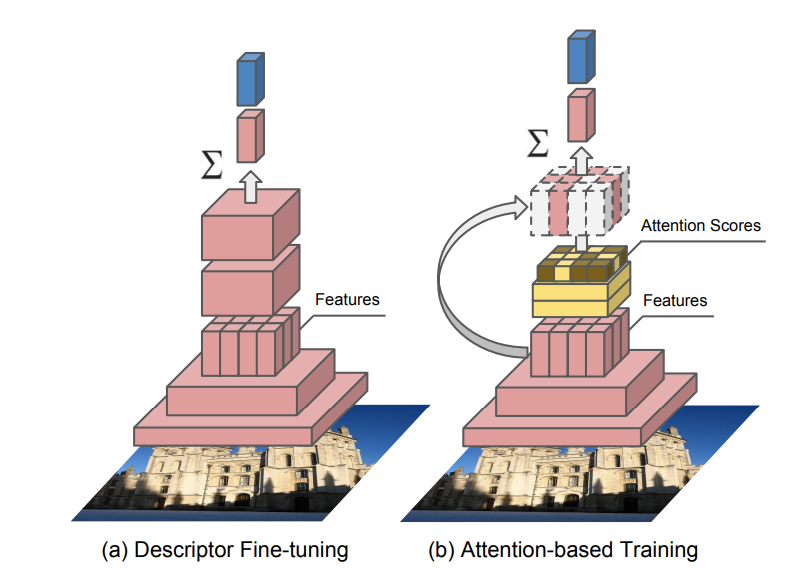
This allows us to extract local features from the input image and then use RANSAC for geometric verification. Random Sample Consensus (RANSAC) is a method to smooth data containing a significant percentage of errors, which is ideally suited for applications in automated image analysis where interpretation is based on the data generated by error-prone feature detectors. The goal of the project is to describe a method for accurate and fast large-scale landmark recognition using the advantages of deep convolutional neural networks.
Methodology
This section will describe in detail the CNN architecture, loss function, training procedure, and inference implementation of the landmark recognition system. The figure below is an overview of the landmark recognition system.

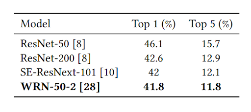
The landmark CNN consists of three parts: the main network, the embedding layer and the classification layer. To obtain a CNN main network suitable for training landmark recognition model, fine-tuning is applied and several pre-trained backbones (Residual Networks) based on other similar datasets, including ResNet-50, ResNet-200, SE-ResNext-101 and Wide Residual Network (WRN-50-2), are evaluated based on inference quality and efficiency, displayed in the table below. Residual networks are shallower architectures compared to usual deep networks and have their layers fit residuals mappings, [math]\displaystyle{ \mathcal{F}(x):= \mathcal{H}(x)-x }[/math]. The residual mappings are then recast into [math]\displaystyle{ \mathcal{F}(x)+x }[/math]. This is realized using shortcut connections to skip various layers and having the outputs added to the outputs of the stacked layers (He, Zhang, Ren, & Sun, 2016). Based on the evaluation results, WRN-50-2 is selected as the optimal backbone architecture. Fine-tuning is a very efficient technique in various computer vision applications because we can take advantage of everything the model has already learned and applied it to our specific task.
For the embedding layer, as shown in the below figure, the last fully-connected layer after the averaging pool is removed. Instead, a fully-connected 2048 [math]\displaystyle{ \times }[/math] 512 layer and a batch normalization layer is added as the embedding layer. After the batch normalization, a fully-connected 512 [math]\displaystyle{ \times }[/math] n layer is added as the classification layer. The below figure shows the overview of the CNN architecture of the landmark recognition system.

To effectively determine the embedding vectors for each landmark class (centroids), the network needs to be trained to have the members of each class to be as close as possible to the centroids. Several suitable loss functions are evaluated including Contrastive Loss, Arcface, and Center loss. The center loss is selected since it achieves the optimal test results and it trains a center of embeddings of each class and penalizes distances between image embeddings as well as their class centers. In addition, the center loss is a simple addition to softmax loss and is trivial to implement.
When implementing the loss function, a new additional class that includes all non-landmark instances needs to be added. The size of the non-landmark class is much greater than the classes of landmarks, and the non-landmark class would not have a specific structure because the non-landmark class contains all other objects. Hence the center loss function needs to be modified to focus on the landmark classes as followed. Let n be the number of landmark classes, m be the mini-batch size, [math]\displaystyle{ x_i \in R^d }[/math] is the i-th embedding and [math]\displaystyle{ y_i }[/math] is the corresponding label where [math]\displaystyle{ y_i \in }[/math] {1,...,n,n+1}, n+1 is the label of the non-landmark class. Denote [math]\displaystyle{ W \in R^{d \times n} }[/math] as the weights of the classifier layer, [math]\displaystyle{ W_j }[/math] as its j-th column. Let [math]\displaystyle{ c_{y_i} }[/math] be the [math]\displaystyle{ y_i }[/math] th embeddings center from Center loss and [math]\displaystyle{ \lambda }[/math] be the balancing parameter of Center loss. Then the final loss function will be:

In the training procedure, the stochastic gradient descent(SGD) will be used as the optimizer with momentum=0.9 and weight decay = 5e-3. For the center loss function, the parameter [math]\displaystyle{ \lambda }[/math] is set to 5e-5. Each image is resized to 256 [math]\displaystyle{ \times }[/math] 256 and several data augmentations are applied to the dataset including random resized crop, color jitter, and random flip. The training dataset is divided into four parts based on the geographical affiliation of cities where landmarks are located: Europe/Russia, North America/Australia/Oceania, the Middle East/North Africa, and the Far East Regions.
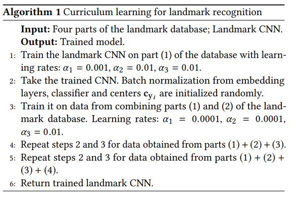
The paper introduces curriculum learning for landmark recognition, which is shown in the below figure. The algorithm is trained for 30 epochs and the learning rate [math]\displaystyle{ \alpha_1, \alpha_2, \alpha_3 }[/math] will be reduced by a factor of 10 at the 12th epoch and 24th epoch.
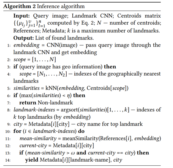
In the inference phase, the paper introduces the term “centroids” which are embedding vectors that are calculated by averaging embeddings and are used to describe landmark classes. The calculation of centroids is significant to effectively determine whether a query image contains a landmark. The paper proposes two approaches to help the inference algorithm to calculate the centroids. First, instead of using the entire training data for each landmark, data cleaning is done to remove most of the redundant and irrelevant elements in the image. For example, if the landmark we are interested in is a palace located on a city square, then images of a similar building on the same square are included in the data which can affect the centroids. Second, since each landmark can have different shooting angles, it is more efficient to calculate a separate centroid for each shooting angle. Hence, a hierarchical agglomerative clustering algorithm is proposed to partition training data into several valid clusters for each landmark and the set of centroids for a landmark L can be represented by [math]\displaystyle{ \mu_{l_j} = \frac{1}{|C_j|} \sum_{i \in C_j} x_i, j \in 1,...,v }[/math] where v is the number of valid clusters for landmark L and v=1 if there is no valid clusters for L.
Once the centroids are calculated for each landmark class, the system can make decisions whether there is a landmark in an image. The query image is passed through the landmark CNN and the resulting embedding vector is compared with all centroids by dot product similarity using approximate k-nearest neighbors (AKNN). To distinguish landmark classes from non-landmark, a threshold [math]\displaystyle{ \eta }[/math] is set and it will be compared with the maximum similarity to determine if the image contains any landmarks.
The full inference algorithm is described in the below figure.
We will now look at how the landmark database was created. The collection process was structured by countries, cities and landmarks. They divided the world into several regions: Europe, America, Middle East, Africa, Far East, Australia and Oceania. Within each region, cities were selected that contained a lot of significant landmarks, and some natural landmarks were filtered out as they are difficult to distinguish. These include landmarks such as parks and beaches, unless they're very notable and popular, for example Santa Monica Pier. Natural landmarks Once the cities and landmarks were selected, both images and metadata were collected for each landmark.
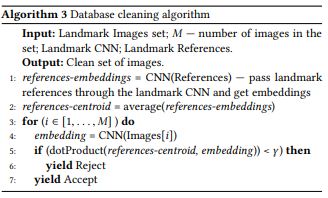
After forming the database, it had to be cleaned before it could be used to train the CNN. First, for each landmark, any redundant images were removed. Then, for each landmark, 5 images were picked that had a high probability of containing the landmark and were checked manually. The database was then cleaned by parts using the curriculum learning process. For each landmark, the centroid was calculated from the references. The centroid is compared to each image of the current landmark data using dot product similarity, and if it is less than the currenbt threshold [math]\displaystyle{ \gamma }[/math] the image is rejected. It is further described in the pseudocode above. The final database contained 11381 landmarks in 503 cities and 70 countries. With 2331784 landmark images and 900,000 non-landmark images. The number of landmarks that have less than 100 images is called "rare".
Experiments and Analysis
Offline test
In order to measure the quality of the model, an offline test set was collected and manually labeled. According to the calculations, photos containing landmarks make up 1 − 3% of the total number of photos on average. This distribution was emulated in an offline test, and the geo-information and landmark references weren’t used. The results of this test are presented in the table below. Two metrics were used to measure the results of experiments: Sensitivity — the accuracy of a model on images with landmarks (also called Recall) and Specificity — the accuracy of a model on images without landmarks. Several types of DELF were evaluated, and the best results in terms of sensitivity and specificity were included in the table below. The table also contains the results of the model trained only with Softmax loss, Softmax, and Center loss. Thus, the table below reflects improvements in our approach with the addition of new elements in it.
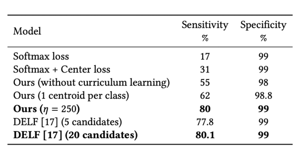
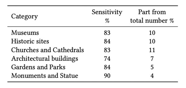
It's very important to understand how a model works on “rare” landmarks due to the small amount of data for them. Therefore, the behavior of the model was examined separately on “rare” and “frequent” landmarks in the table below. The column “Part from total number” shows what percentage of landmark examples in the offline test has the corresponding type of landmarks. And we find that the sensitivity of “frequent” landmarks is much higher than “rare” landmarks.

Analysis of the behavior of the model in different categories of landmarks in the offline test is presented in the table below. These results show that the model can successfully work with various categories of landmarks. Predictably better results (92% of sensitivity and 99.5% of specificity) could also be obtained when the offline test with geo-information was launched on the model.
Revisited Paris dataset
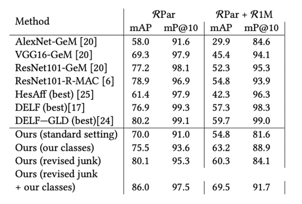
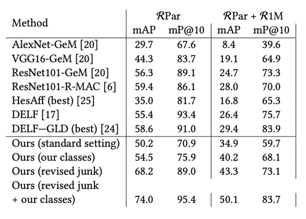
Revisited Paris dataset (RPar)[2] was also used to measure the quality of the landmark recognition approach. This dataset with Revisited Oxford (ROxf) is standard benchmarks for the comparison of image retrieval algorithms. In recognition, it is important to determine the landmark, which is contained in the query image. Images of the same landmark can have different shooting angles or taken inside/outside the building. Thus, it is reasonable to measure the quality of the model in the standard and adapt it to the task settings. That means not all classes from queries are presented in the landmark dataset. For those images containing correct landmarks but taken from different shooting angles within the building, we transferred them to the “junk” category, which does not influence the final score and makes the test markup closer to our model’s goal. Results on RPar with and without distractors in medium and hard modes are presented in the table below.
Comparison
Recent most efficient approaches to landmark recognition are built on fine-tuned CNN. We chose to compare our method to DELF on how well each performs on recognition tasks. A brief summary is given below:

Offline test and timing
Both approaches obtained similar results for image retrieval in the offline test (shown in the sensitivity&specificity table), but the proposed approach is much faster on the inference stage and more memory efficient.
To be more detailed, during the inference stage, DELF needs more forward passes through CNN, has to search the entire database, and performs the RANSAC method for geometric verification. All of them make it much more time-consuming than our proposed approach. Our approach mainly uses centroids, this makes it take less time and needs to store fewer elements.
Conclusion
In this paper, we were hoping to solve some difficulties that emerge when trying to apply landmark recognition with a scalable approach to the production level, which is the kind of implementation that has been deployed to production at scale and used for recognition of user photos in the Mail.ru cloud application: there might not be a clean & sufficiently large database for interesting tasks, algorithms should be fast, scalable, and should aim for low FP and high accuracy. The basis of this method is the use of embedded deep convolutional neural networks. The CNN is trained through course learning techniques and has a modified version of the center loss. To determine whether there are a landmark image embedding vector and one or more centroids of each class on the given image.
While aiming for these goals, we presented a way of cleaning landmark data. And most importantly, we introduced the usage of embeddings of deep CNN to make recognition fast and scalable, trained by curriculum learning techniques with modified versions of Center loss. Compared to the state-of-the-art methods, this approach shows similar results but is much faster and suitable for implementation on a large scale.
Critique
The paper selected 5 images per landmark and checked them manually. That means the training process takes a long time on data cleaning and so the proposed algorithm lacks reusability. Also, since only the landmarks that are the largest and most popular were used to train the CNN, the trained model will probably be most useful in big cities instead of smaller cities with less popular landmarks.
In addition, researchers often look for reliability and reproducibility. By using a private database and manually labeling, it lends itself to an array of issues in terms of validity and integrity. Researchers who are looking for such an algorithm will not be able to sufficiently determine if the experiments do actually yield the claimed results. Also, manual labeling by those who are related to the individuals conducting this research also raises the question of conflict of interest. The primary experiment of this paper should be on public and third-party datasets.
CNN is very similar to ONN (ordinary Neural Networks), each neuron receives some inputs, and then performs a dot product and expresses a single differentiable score function. But what makes CNN interesting is that the neurons are with learnable weights and biases. In this case, it's much easier for us to make some analysis.
It might be worth looking into the ability to generalize better, for example, can this model applied to other structures such as logos, symbols, etc. It would allow a different point of view of how the models perform well or not.
This is a very interesting implementation in some specific field. The paper shows a process to analyze the problem and trains the model based on deep CNN implementation. In future work, it would be some practical advice to compare the deep CNN model with other models. By comparison, we might receive a more comprehensive training model for landmark recognition.
This summary has a good structure and the methodology part is very clear for readers to understand. Using some diagrams for the comparison with other methods is good for visualization for readers. Since the dataset is marked manually, so it is kind of time-consuming for training a model. So it might be interesting to discuss how the famous IT company (i.e. Google etc.) fix this problem.
It would be beneficial if the authors could provide more explanations regarding the DELF method. Visualization of the differences between DELF and CNN from an algorithm and architecture perspective would be highly significant for the context of this paper.
One challenge of landmark recognition is a large number of classes. It would be good to see the comparison between the proposed model and other models in terms of efficiency.
The scope of this paper seems to work specifically with some of the most well-known landmarks in the world, and many of these landmarks are well known because they are very distinct in how they look. It would be interesting to see how well the model works when classifying different landmarks of similar type (ie, Notre Dame Cathedral vs. St. Paul's Cathedral, etc.). It would also be interesting to see how this model compares with other models in the literature, or if this is unique, perhaps the authors could scale this model down to a landmark classification problem (castles, churches, parks, etc.) and compare it against other models that way.
Paper 25 (Loss Function Search in Facial Recognition) also utilizes the softmax loss function in feature discrimination in images. The difference between this paper and paper 25 is that this paper focuses on landmark images, whereas paper 25 is on facial recognition. Despite the slightly different application, both papers prove the importance of using the softmax loss function in feature discrimination, which is pretty neat. Since both papers use softmax loss function for image recognition, it will be interesting to apply it to a dataset where both a landmark and human face are present, for example, photos on Instagram. Since Instagram users usually tag the landmark, supervised learning methods such as a multi-task learning model can be easily applied to the dataset. (See paper 14)
The paper uses typical representatives of landmarks in various continents during training. It would be interesting to see how different results would be if the average structure of all landmarks present were used.
The curriculum learning algorithm categories the landmarks into four different geographical locations, i.e (1) Europe, (2) North America, Australia and Oceania; (3) Middle East, North Africa; (4) Far east, because landmarks from the same geographical locations are similar to each other than from different geographical locations. Landmarks can also be categorized into archeological landmarks like medieval castles, architectural landmarks like monuments, biological landmarks like some parks or gardens, geological landmarks like caves etc, and it would be interesting to explore what kinds of results the curriculum learning algorithm would produce if the landmarks were categorized in different ways. Also In paper 17, i.e poker AI, uses an approach where similar decision points in the game were grouped together in a process called abstraction. Therefore a similar kind of approach of grouping objects is used in the methods described in both papers which indeed helps in reducing the computational time and makes the process more scalable.
Given that the curriculum learning method in the paper has 4 categories that divide the data into continents, would adding more categories increase the accuracy of the algorithm? For instance, by using the continent information and meta-data from images, and even the lighting of the images, it may be possible to determine more detailed location data of the images. Also, what about landmarks that do not conform to the "style" of architecture in a continent? Are landmarks of "styles" that are less common in all of the continents more difficult to identify with this algorithm?
Authors have outlined 3 potential problems but they did not explain how to fix them. It's better to specify how can we handle these problems otherwise we cannot apply this model to the real world problems. For example, the real world problems always have big training data and the content might not be clean.
I got an impression that it works on a Large Scale Landmark Dataset from the title. However it does not mention anything about the process or proof that it can efficiently and accurately classify a large landmarks dataset. It was also only mentioned that the first dataset was "collected and manually labeled", but does not mention how it was collected. The second dataset was landmarks in Paris. If the author were to tune the model only according to these data, it is obvious that it can not be generalized well. It might be able to classify landmarks at where the images in dataset are taken or landmarks in Paris, but it might not work in other areas that has different culture, where the landmarks might look very different.
It would be better that if the summary have an extended usage of the model. For instance, if this model can applied to any other aspects rather than landmark recognition. It will give us a more general understanding of the model.
It is really important that all the data comes from one format, such as all comes from an image. Because sometimes it is really expensive to go scan the land structure in person, and the form of images is more common. So it is better that the author can focus on one form so that cleaner data can be captured.
In the introduction, it was claimed that the deep CNN could be used in an online fashion due to its efficiency. It would be better if the author could provide a benchmark of existing methods and the model given in this paper in an online fashion to compare their accuracy and efficiency.
References
[1] Andrei Boiarov and Eduard Tyantov. 2019. Large Scale Landmark Recognition via Deep Metric Learning. In The 28th ACM International Conference on Information and Knowledge Management (CIKM ’19), November 3–7, 2019, Beijing, China. ACM, New York, NY, USA, 10 pages. https://arxiv.org/pdf/1908.10192.pdf 3357384.3357956
[2] FilipRadenović,AhmetIscen,GiorgosTolias,YannisAvrithis,andOndřejChum. 2018. Revisiting Oxford and Paris: Large-Scale Image Retrieval Benchmarking. arXiv preprint arXiv:1803.11285 (2018).
[3] He, K., Zhang, X., Ren, S., & Sun, J. (2016). Deep Residual Learning for Image Recognition. 2016 IEEE Conference on Computer Vision and Pattern Recognition (CVPR), 770-771. doi:10.1109/cvpr.2016.90