Synthesizing Programs for Images usingReinforced Adversarial Learning: Difference between revisions
No edit summary |
|||
| (106 intermediate revisions by 15 users not shown) | |||
| Line 1: | Line 1: | ||
'''Synthesizing Programs for Images | '''Synthesizing Programs for Images using Reinforced Adversarial Learning: ''' Summary of the ICML 2018 paper | ||
Paper: [[http://proceedings.mlr.press/v80/ganin18a.html]] | |||
Video: [[https://www.youtube.com/watch?v=iSyvwAwa7vk&feature=youtu.be]] | |||
== Presented by == | == Presented by == | ||
| Line 5: | Line 8: | ||
1. Nekoei, Hadi [Quest ID: 20727088] | 1. Nekoei, Hadi [Quest ID: 20727088] | ||
= Motivation = | |||
Conventional neural generative models have major problems. | Conventional neural generative models have major problems. | ||
* | * It is not clear how to inject knowledge about the data into the model. | ||
* | * Latent space is not easily interpretative. | ||
The provided solution in this paper is to generate programs to incorporate tools, e.g. graphics editors, illustration software, CAD. and '''creating more meaningful API(sequence of complex actions vs raw pixels)'''. | The provided solution in this paper is to generate programs to incorporate tools, e.g. graphics editors, illustration software, CAD. and '''creating more meaningful API(sequence of complex actions vs raw pixels)'''. | ||
= Introduction = | |||
Humans, frequently, use the ability to recover structured representation from raw sensation to understand their environment. Decomposing a picture of a hand-written character into strokes or understanding the layout of a building can be exploited to learn how actually our brain works. | |||
In the visual domain, inversion of a renderer for the purposes of scene understanding is typically referred to as inverse graphics. However, training vision systems using the inverse graphics approach has remained a challenge. Renderers typically expect as input programs that have sequential semantics, are composed of discrete symbols (e.g., keystrokes in a CAD program), and are long (tens or hundreds of symbols). Additionally, matching rendered images to real data poses an optimization problem as black-box graphics simulators are not differentiable in general. | |||
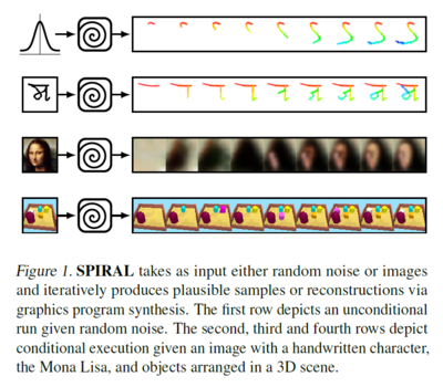
To address these problems, a new approach is presented for interpreting and generating images using Deep Reinforced Adversarial Learning in order to solve the need for a large amount of supervision and scalability to larger real-world datasets. In this approach, an adversarially trained agent '''(SPIRAL)''' generates a program which is executed by a graphics engine to generate images, either conditioned on data or unconditionally. The agent is rewarded by fooling a discriminator network and is trained with distributed reinforcement learning without any extra supervision. The discriminator network itself is trained to distinguish between generated and real images. | To address these problems, a new approach is presented for interpreting and generating images using Deep Reinforced Adversarial Learning in order to solve the need for a large amount of supervision and scalability to larger real-world datasets. In this approach, an adversarially trained agent '''(SPIRAL)''' generates a program which is executed by a graphics engine to generate images, either conditioned on data or unconditionally. The agent is rewarded by fooling a discriminator network and is trained with distributed reinforcement learning without any extra supervision. The discriminator network itself is trained to distinguish between generated and real images. | ||
[[File:Fig1 SPIRAL.PNG | 400px | [[File:Fig1 SPIRAL.PNG | 400px|center]] | ||
== Related Work == | == Related Work == | ||
| Line 40: | Line 46: | ||
* Lack the ability to infer structured representations of images | * Lack the ability to infer structured representations of images | ||
= The SPIRAL Agent = | |||
=== Overview === | === Overview === | ||
The paper aims to construct a generative model <math>\mathbf{G}</math> to take samples from a distribution <math>p_{d}</math>. The generative model consists of a recurrent network <math>\pi</math> (called policy network or agent) and an external rendering simulator R that accepts a sequence of commands from the agent and maps them into the domain of interest, e.g. R could be a CAD program rendering descriptions of primitives into 3D scenes. | The paper aims to construct a generative model <math>\mathbf{G}</math> to take samples from a distribution <math>p_{d}</math>. The generative model consists of a recurrent network <math>\pi</math> (called policy network or agent) and an external rendering simulator R that accepts a sequence of commands from the agent and maps them into the domain of interest, e.g. R could be a CAD program rendering descriptions of primitives into 3D scenes. | ||
In order to train policy network <math>\pi</math>, the paper has exploited generative adversarial network. In this framework, the generator tries to fool a discriminator network which is trained to distinguish between real and fake samples. Thus, the distribution generated by <math>\mathbf{G}</math> approaches <math> | In order to train policy network <math>\pi</math>, the paper has exploited generative adversarial network. In this framework, the generator tries to fool a discriminator network which is trained to distinguish between real and fake samples. Thus, the distribution generated by <math>\mathbf{G}</math> approaches <math>p_d</math>. | ||
== Objectives == | |||
The authors give training objective for <math>\mathbf{G}</math> and <math>\mathbf{D}</math> as follows. | The authors give training objective for <math>\mathbf{G}</math> and <math>\mathbf{D}</math> as follows. | ||
'''Discriminator:''' Following (Gulrajani et al., 2017), the objective for <math>\mathbf{D}</math> is defined as: | '''Discriminator:''' Following (Gulrajani et al., 2017), the objective for <math>\mathbf{D}</math> is defined as: | ||
\begin{align} | |||
\mathcal{L}_D = -\mathbb{E}_{x\sim p_d}[D(x)] + \mathbb{E}_{x\sim p_g}[D(x)] + R | |||
\end{align} | |||
where <math>\mathbf{R}</math> is a regularization term softly constraining <math>\mathbf{D}</math> to stay in the set of Lipschitz continuous functions (for some fixed Lipschitz constant). | where <math>\mathbf{R}</math> is a regularization term softly constraining <math>\mathbf{D}</math> to stay in the set of Lipschitz continuous functions (for some fixed Lipschitz constant). | ||
| Line 57: | Line 65: | ||
\begin{align} | |||
\mathcal{L}_G = -\sum_{t}\log\pi(a_t|s_t;\theta)[R_t - V^{\pi}(s_t)] | |||
\end{align} | |||
where <math>V^{\pi}</math> is an approximation to the value function which is considered to be independent of theta, and <math>R_{t} = \sum_{t}^{N}r_{t}</math> is a | where <math>V^{\pi}</math> is an approximation to the value function which is considered to be independent of theta, and <math>R_{t} = \sum_{t}^{N}r_{t}</math> is a | ||
1-sample Monte-Carlo estimate of the return. Rewards are set to: | 1-sample Monte-Carlo estimate of the return. Rewards are set to: | ||
<math> | <math> | ||
r_t = \begin{cases} | |||
0 & \text{for } t < N \\ | |||
D(\mathcal{R}(a_1, a_2, \cdots, a_N)) & \text{for } t = N | |||
\end{cases} | |||
</math> | </math> | ||
One interesting aspect of this new formulation is that | |||
One interesting aspect of this new formulation is that | |||
the search can be biased by introducing intermediate rewards | |||
which may depend not only on the output of R but also on | which may depend not only on the output of R but also on | ||
commands used to generate that output. | commands used to generate that output. | ||
== Conditional generation: == | |||
In some cases such as producing a given image <math>x_{target}</math>, conditioning the model on auxiliary inputs is useful. That can be done by feeding <math>x_{target}</math> to both policy and discriminator networks as: | In some cases such as producing a given image <math>x_{target}</math>, conditioning the model on auxiliary inputs is useful. That can be done by feeding <math>x_{target}</math> to both policy and discriminator networks as: | ||
<math> | <math> | ||
p_g = | p_g = R(p_a(a|x_{target})) | ||
</math> | </math> | ||
=== Distributed Learning: | While <math>p_{d}</math> becomes a Dirac-<math>\delta</math> function centered at <math>x_{target}</math>. | ||
For the first two terms in the objective function for D, they reduce to | |||
<math> | |||
-D(x_{target}|x_{target})+ \mathbb{E}_{x\sim p_g}[D(x|x_{target})] | |||
</math> | |||
It can be proven that for this particular setting of <math>p_{g}</math> and <math>p_{d}</math>, the <math>l2</math>-distance is an optimal discriminator. It may be as a poor candidate for the reward signal of the generator, even if it is not the only solution of the objective function for D. | |||
===Traditional GAN generation: === | |||
Traditional GANs use the following minimax objective function to quantify optimality for relationships between D and G: | |||
[[File:edit7.png| 400px|center]] | |||
Minimizing the Jensen-Shannon divergence between the two distribution often leads to vanishing gradients as the discriminator saturates. We circumvent this issue using the conditional generation function, which is much better behaved. | |||
== Distributed Learning: == | |||
The training pipeline is outlined in Figure 2b. It is an extension of the recently proposed '''IMPALA''' architecture (Espeholt et al., 2018). For training, three kinds of workers are defined: | |||
| Line 92: | Line 116: | ||
* A policy learner receives trajectories from the actors, combines them into a batch and updates <math>\pi</math> by performing '''SGD''' step on <math>\mathcal{L}_G</math> (2). Following common practice (Mnih et al., 2016), | * A policy learner receives trajectories from the actors, combines them into a batch and updates <math>\pi</math> by performing '''SGD''' step on <math>\mathcal{L}_G</math> (2). Following common practice (Mnih et al., 2016), <math>\mathcal{L}_G</math> is augmented with an entropy penalty encouraging exploration. | ||
* In contrast to the base '''IMPALA''' setup, | * In contrast to the base '''IMPALA''' setup, an additional discriminator learner is defined. This worker consumes random examples from <math>p_{d}</math>, as well as generated data (final renders) coming from the actor workers, and optimizes <math>\mathcal{L}_D</math> (1). | ||
random examples from <math>p_{d}</math>, as well as generated data (final renders) coming from the actor workers, and optimizes <math>\mathcal{L}_D</math> (1). | |||
[[File:Fig2 SPIRAL Architecture.png | 700px|center]] | |||
'''Note:''' no trajectories are omitted in the policy learner. Instead, the <math>D</math> updates is decoupled from the <math>\pi</math> updates by introducing a replay buffer that serves as a communication layer between the actors and the discriminator learner. That allows the latter to optimize <math>D</math> at a higher rate than the training of the policy network due to the difference in network sizes (<math>\pi</math> is a multi-step RNN, while <math>D</math> is a plain '''CNN'''). Even though sampling from a replay buffer inevitably results in smoothing of <math>p_{g}</math>, this setup is found to work well in practice. | |||
= Experiments= | |||
== Environments == | |||
Two rendering environment is introduced. For MNIST, OMNIGLOT and CELEBA generation an open-source painting librabry LIMBYPAINT (libmypaint | Two rendering environment is introduced. For MNIST, OMNIGLOT and CELEBA generation an open-source painting librabry LIMBYPAINT (libmypaint | ||
contributors, 2018).) is used. The agent controls a brush and produces | contributors, 2018).) is used. The agent controls a brush and produces | ||
a sequence of (possibly disjoint) strokes on a canvas | a sequence of (possibly disjoint) strokes on a canvas | ||
C. The state of the environment is comprised of the contents | C. The state of the environment is comprised of the contents | ||
of | of <math>C</math> as well as the current brush location <math>l_{t}</math>. Each action | ||
<math>a_{t}</math> is a tuple of 8 discrete decisions <math>(a_t^1; a_t^2; ... ; a_t^8)</math> (see | |||
Figure 3). The first two components are the control point | Figure 3). The first two components are the control point <math>p_{c}</math> | ||
and the | and the endpoint <math>l_{t+1}</math> of the stroke. | ||
[[File:Fig3_agent_action_space.PNG | 450px|center]] | |||
The next 5 | The next 5 | ||
components represent the appearance of the stroke: the | components represent the appearance of the stroke: the | ||
pressure that the agent applies to the brush (10 levels), the | pressure that the agent applies to the brush (10 levels), the | ||
brush size, and the stroke color characterized by mixture | brush size, and the stroke color characterized by a mixture | ||
of red, green and blue (20 bins for each color component). | of red, green and blue (20 bins for each color component). | ||
The last element of at is a binary flag specifying the type | The last element of at is a binary flag specifying the type | ||
of action: the agent can choose either to produce a stroke | of action: the agent can choose either to produce a stroke | ||
or to jump right to | or to jump right to <math>l_{t+1}</math>. | ||
In the MUJOCO SCENES experiment, we render images | In the MUJOCO SCENES experiment, we render images | ||
using a MuJoCo-based environment (Todorov et al., 2012). | using a MuJoCo-based environment (Todorov et al., 2012). | ||
At each time step, the agent has to decide on the object | At each time step, the agent has to decide on the object | ||
type (4 options), its location on a 16 | type (4 options), its location on a 16 <math>\times</math> 16 grid, its size | ||
(3 options) and the color (3 color components with 4 bins | (3 options) and the color (3 color components with 4 bins | ||
each). The resulting tuple is sent to the environment, which | each). The resulting tuple is sent to the environment, which | ||
adds an object to the scene according to the specification. | adds an object to the scene according to the specification. | ||
== Datasets == | |||
=== MNIST === | === MNIST === | ||
For the MNIST dataset, two sets of experiments | For the MNIST dataset, two sets of experiments are conducted: | ||
1- In this experiment, an unconditional agent is trained to model the data distribution. Along with the reward provided by discriminator, a small negative reward is provided to the agent for each continuous sequence of strokes to encourage the agent to draw a digit in a continuous motion of stroke. Example of such generation is depicted in the Fig 4a. | 1- In this experiment, an unconditional agent is trained to model the data distribution. Along with the reward provided by the discriminator, a small negative reward is provided to the agent for each continuous sequence of strokes to encourage the agent to draw a digit in a continuous motion of stroke. Example of such generation is depicted in the Fig 4a. | ||
2- In the second experiment, an agent is trained to reproduce a given digit. | 2- In the second experiment, an agent is trained to reproduce a given digit. | ||
Several examples of conditional generated digits | Several examples of conditional generated digits are shown in Fig 4b. | ||
[[File:Fig4a MNIST.png | 450px|center]] | |||
=== OMNIGLOT === | === OMNIGLOT === | ||
Now the trained agents | Now the trained agents are tested in a similar but more challenging setting of handwritten characters. As can be seen in Fig 5a, the unconditional generation has a lower quality compared to digits in the previous dataset. The conditional agents, on the other hand, were able to reach a convincing quality (Fig 5b). Moreover, as OMNIGLOT has lots of different symbols, the model that we created was able to learn a general idea of image production without memorizing the training data. We tested this result by inputting new unseen line drawings to our trained agent. As we concluded, it provided excellent results as shown in Figure 6. | ||
[[File:Fig5 OMNIGLOT.png | 450px|center]] | |||
For the MNIST dataset, two kinds of rewards, discriminator score and | For the MNIST dataset, two kinds of rewards, discriminator score and <math>l^{2}-\text{distance}</math> has been compared. Note that the discriminator based approach has a significantly lower training time and lower final <math>l^{2}</math> error. | ||
Following (Sharma et al., 2017), also a “blind” version | Following (Sharma et al., 2017), also a “blind” version of the agent without feeding any intermediate canvas states as an input to <math>\pi</math> is trained. The training curve for this experiment is also reported in Fig 8a. | ||
of the agent without feeding any intermediate canvas | (dotted blue line) The results of training agents with discriminator based and <math>l^{2}-\text{distance}</math> approach is shown in Fig 8a as well. | ||
states as an input to | |||
=== CELEBA === | === CELEBA === | ||
Since the libmypaint environment is also capable of producing | Since the ''libmypaint'' environment is also capable of producing | ||
complex color paintings, | complex color paintings, this direction is explored by | ||
training a conditional agent on the CELEBA dataset. In this | training a conditional agent on the CELEBA dataset. In this | ||
experiment, the agent does not receive any intermediate rewards. | experiment, the agent does not receive any intermediate rewards. | ||
In addition to the reconstruction reward (either | In addition to the reconstruction reward (either <math>l^2</math> or | ||
discriminator-based), | discriminator-based), earth mover’s | ||
distance between the color histograms of the model’s output | distance between the color histograms of the model’s output | ||
and | and <math>x_{target}</math> is penalized. (Figure 7) | ||
[[File:Fig6 CELEBA.png | 450px|center]] | |||
Although blurry, the model’s reconstruction closely matches | Although blurry, the model’s reconstruction closely matches | ||
the high-level structure of each image | the high-level structure of each image such as the | ||
background color, the position of the face and the color of | background color, the position of the face, and the color of | ||
the person’s hair. In some cases, shadows around eyes and | the person’s hair. In some cases, shadows around eyes and | ||
the nose | the nose is visible. | ||
For the MUJOCO SCENES dataset, | === MUJOCO SCENES === | ||
simple CAD programs that best explain input images. | |||
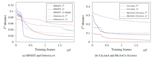
Here | For the MUJOCO SCENES dataset, the trained agent is used to construct simple CAD programs that best explain input images. Here only the case of the conditional generation is considered. Like before, the reward function for the generator can be either the <math>l^2</math> score or the discriminator output. In addition, there are not any auxiliary reward signals. This model has the capacity to infer and represent up to 20 objects and their attributes due to its unrolled 20 time steps. | ||
Like before, the reward function for the generator can | |||
be either the | |||
As shown in Figure 8b, the agent trained to directly minimize | As shown in Figure 8b, the agent trained to directly minimize | ||
<math>l^2</math> is unable to solve the task and has significantly | |||
higher pixel-wise error. In comparison, the | higher pixel-wise error. In comparison, the discriminator based | ||
variant solves the task and produces near-perfect reconstructions | variant solves the task and produces near-perfect reconstructions | ||
on a holdout set (Figure 10). | on a holdout set (Figure 10). | ||
[[File:Fig8 MUJOCO_SCENES.png | 500px|center]] | |||
For this experiment, the total number of possible execution traces is <math>M^N</math>, where <math>M = 4·16^2·3·4^3·3 </math> is the total number of attribute settings for a single object and N = 20 is the length of an episode. Then a general-purpose Metropolis-Hastings inference algorithm that samples an execution trace defining attributes for a maximum of 20 primitives was run on a set of 100 images. These attributes are considered as latent variables. During each time step of the inference, the attribute blocks (including presence/absence tags) corresponding to a single object are evenly flipped over the appropriate range. The resulting trace is presented as an output sample by the environment and then the output sample is accepted or rejected using the Metropolis-Hastings update rule, where the Gaussian likelihood is centered on the test image and the fixed diagonal covariance is 0.25. From Figure 9, the MCMC search baseline cannot solve the task even after a lot of evaluation. | |||
[[File:figure9 mcmc.PNG| 500px|center]] | |||
= Discussion = | |||
As in the OMNIGLOT | As in the OMNIGLOT | ||
experiment, the | experiment, the <math>l^2</math>-based agent demonstrates some | ||
improvements over the random policy but gets stuck and as | |||
a result | a result fails to learn sensible reconstructions (Figure 8b). | ||
[[File:Fig7 Results.png | 500px|center]] | |||
Scaling visual program synthesis to real world and combinatorial | |||
datasets has been a challenge. | Scaling visual program synthesis to the real world and combinatorial | ||
black-box rendering | datasets has been a challenge. It has been shown that it is possible to train an adversarial generative agent employing | ||
black-box rendering simulator. Our results indicate that | |||
using the Wasserstein discriminator’s output as a reward | using the Wasserstein discriminator’s output as a reward | ||
function with asynchronous reinforcement learning can provide | function with asynchronous reinforcement learning can provide | ||
a scaling path for visual program synthesis. The current | a scaling path for visual program synthesis. The current | ||
exploration strategy used in the agent is entropy-based | exploration strategy used in the agent is entropy-based but | ||
future work should address this limitation by employing sophisticated | future work should address this limitation by employing sophisticated | ||
search algorithms for policy improvement. For | search algorithms for policy improvement. For | ||
| Line 217: | Line 234: | ||
inference algorithms could also be used for this purpose. | inference algorithms could also be used for this purpose. | ||
= | = Critique and Future Work = | ||
Future work should explore different parameterizations of | * The architecture isn't new but it's a nice application and it's fun to watch the video of the robot painting in real life. SPIRAL's GAN-like idea continues the vein of [https://arxiv.org/abs/1610.01945 connecting actor-critic RL with GANs] like " [https://arxiv.org/abs/1706.03741Deep reinforcement learning from human preferences]" , Christiano et al 2017 or GAIL: | ||
action spaces. For instance, the use of two arbitrary control | |||
points is perhaps not the best way to represent strokes, as it | * Future work should explore different parameterizations of action spaces. For instance, the use of two arbitrary control points is perhaps not the best way to represent strokes, as it is hard to deal with straight lines. Actions could also directly parametrize 3D surfaces, planes, and learned texture models to invert richer visual scenes. | ||
is hard to deal with straight lines. Actions could also directly parametrize 3D surfaces, planes and learned texture models | |||
to invert richer visual scenes. On the reward side, using | * A potential application can be in the field of medical images specifically to enhance and recolor histopathology slides for better detection. Also, image restoration problems could be addressed based on these approaches. | ||
a joint image-action discriminator similar to BiGAN/ALI | |||
(Donahue et al., 2016; Dumoulin et al., 2016) (in this case, | * On the reward side, using a joint image-action discriminator similar to BiGAN/ALI (Donahue et al., 2016; Dumoulin et al., 2016) (in this case, the policy can be viewed as an encoder, while the renderer becomes a decoder) could result in a more meaningful learning signal, since D will be forced to focus on the semantics of the image. | ||
the policy can viewed as an encoder, while the renderer becomes | |||
a decoder) could result in a more meaningful learning | * The paper could also provide an avenue to further explore inverse simulation and program synthesis on applications ranging from vision , graphics, speech, music and scientific simulators. | ||
signal, since D will be forced to focus on the semantics of | |||
the | * The paper provides a novel framework for designing and evaluating generative approaches for drawing and painting without explicit supervision. However, more research might be required to design a proper reward function for each specific domain. For some applications can be beneficial to let the actor explore a wider number of alternatives without applying a penalization for using more drawing movements. In other words, by leaving the actor work in a wider search space, some sort of creativity could emerge and newer or better procedures might be discovered. | ||
= Other Resources = | |||
#Code implementation [https://github.com/carpedm20/SPIRAL-tensorflow] | |||
= References = | |||
# Yaroslav Ganin, Tejas Kulkarni, Igor Babuschkin, S.M. Ali Eslami, Oriol Vinyals, [[https://arxiv.org/abs/1804.01118]]. | |||
Latest revision as of 18:31, 16 December 2018
Synthesizing Programs for Images using Reinforced Adversarial Learning: Summary of the ICML 2018 paper
Presented by
1. Nekoei, Hadi [Quest ID: 20727088]
Motivation
Conventional neural generative models have major problems.
- It is not clear how to inject knowledge about the data into the model.
- Latent space is not easily interpretative.
The provided solution in this paper is to generate programs to incorporate tools, e.g. graphics editors, illustration software, CAD. and creating more meaningful API(sequence of complex actions vs raw pixels).
Introduction
Humans, frequently, use the ability to recover structured representation from raw sensation to understand their environment. Decomposing a picture of a hand-written character into strokes or understanding the layout of a building can be exploited to learn how actually our brain works.
In the visual domain, inversion of a renderer for the purposes of scene understanding is typically referred to as inverse graphics. However, training vision systems using the inverse graphics approach has remained a challenge. Renderers typically expect as input programs that have sequential semantics, are composed of discrete symbols (e.g., keystrokes in a CAD program), and are long (tens or hundreds of symbols). Additionally, matching rendered images to real data poses an optimization problem as black-box graphics simulators are not differentiable in general.
To address these problems, a new approach is presented for interpreting and generating images using Deep Reinforced Adversarial Learning in order to solve the need for a large amount of supervision and scalability to larger real-world datasets. In this approach, an adversarially trained agent (SPIRAL) generates a program which is executed by a graphics engine to generate images, either conditioned on data or unconditionally. The agent is rewarded by fooling a discriminator network and is trained with distributed reinforcement learning without any extra supervision. The discriminator network itself is trained to distinguish between generated and real images.
Related Work
Related works in this filed is summarized as follows:
- There has been a huge amount of studies on inverting simulators to interpret images (Nair et al., 2008; Paysan et al., 2009; Mansinghka et al., 2013; Loper & Black, 2014; Kulkarni et al., 2015a; Jampani et al., 2015)
- Inferring motor programs for reconstruction of MNIST digits (Nair & Hinton, 2006)
- Visual program induction in the context of hand-written characters on the OMNIGLOT dataset (Lake et al., 2015)
- inferring and learning feed-forward or recurrent procedures for image generation (LeCun et al., 2015; Hinton & Salakhutdinov, 2006; Goodfellow et al., 2014; Ackley et al., 1987; Kingma & Welling, 2013; Oord et al., 2016; Kulkarni et al., 2015b; Eslami et al., 2016; Reed et al., 2017; Gregor et al., 2015).
However, all of these methods have limitations such as:
- Scaling to larger real-world datasets
- Requiring hand-crafted parses and supervision in the form of sketches and corresponding images
- Lack the ability to infer structured representations of images
The SPIRAL Agent
Overview
The paper aims to construct a generative model [math]\displaystyle{ \mathbf{G} }[/math] to take samples from a distribution [math]\displaystyle{ p_{d} }[/math]. The generative model consists of a recurrent network [math]\displaystyle{ \pi }[/math] (called policy network or agent) and an external rendering simulator R that accepts a sequence of commands from the agent and maps them into the domain of interest, e.g. R could be a CAD program rendering descriptions of primitives into 3D scenes. In order to train policy network [math]\displaystyle{ \pi }[/math], the paper has exploited generative adversarial network. In this framework, the generator tries to fool a discriminator network which is trained to distinguish between real and fake samples. Thus, the distribution generated by [math]\displaystyle{ \mathbf{G} }[/math] approaches [math]\displaystyle{ p_d }[/math].
Objectives
The authors give training objective for [math]\displaystyle{ \mathbf{G} }[/math] and [math]\displaystyle{ \mathbf{D} }[/math] as follows.
Discriminator: Following (Gulrajani et al., 2017), the objective for [math]\displaystyle{ \mathbf{D} }[/math] is defined as:
\begin{align} \mathcal{L}_D = -\mathbb{E}_{x\sim p_d}[D(x)] + \mathbb{E}_{x\sim p_g}[D(x)] + R \end{align}
where [math]\displaystyle{ \mathbf{R} }[/math] is a regularization term softly constraining [math]\displaystyle{ \mathbf{D} }[/math] to stay in the set of Lipschitz continuous functions (for some fixed Lipschitz constant).
Generator: To define the objective for [math]\displaystyle{ \mathbf{G} }[/math], a variant of the REINFORCE (Williams, 1992) algorithm, advantage actor-critic (A2C) is employed:
\begin{align}
\mathcal{L}_G = -\sum_{t}\log\pi(a_t|s_t;\theta)[R_t - V^{\pi}(s_t)]
\end{align}
where [math]\displaystyle{ V^{\pi} }[/math] is an approximation to the value function which is considered to be independent of theta, and [math]\displaystyle{ R_{t} = \sum_{t}^{N}r_{t} }[/math] is a
1-sample Monte-Carlo estimate of the return. Rewards are set to:
[math]\displaystyle{ r_t = \begin{cases} 0 & \text{for } t \lt N \\ D(\mathcal{R}(a_1, a_2, \cdots, a_N)) & \text{for } t = N \end{cases} }[/math]
One interesting aspect of this new formulation is that the search can be biased by introducing intermediate rewards which may depend not only on the output of R but also on commands used to generate that output.
Conditional generation:
In some cases such as producing a given image [math]\displaystyle{ x_{target} }[/math], conditioning the model on auxiliary inputs is useful. That can be done by feeding [math]\displaystyle{ x_{target} }[/math] to both policy and discriminator networks as: [math]\displaystyle{ p_g = R(p_a(a|x_{target})) }[/math]
While [math]\displaystyle{ p_{d} }[/math] becomes a Dirac-[math]\displaystyle{ \delta }[/math] function centered at [math]\displaystyle{ x_{target} }[/math]. For the first two terms in the objective function for D, they reduce to [math]\displaystyle{ -D(x_{target}|x_{target})+ \mathbb{E}_{x\sim p_g}[D(x|x_{target})] }[/math]
It can be proven that for this particular setting of [math]\displaystyle{ p_{g} }[/math] and [math]\displaystyle{ p_{d} }[/math], the [math]\displaystyle{ l2 }[/math]-distance is an optimal discriminator. It may be as a poor candidate for the reward signal of the generator, even if it is not the only solution of the objective function for D.
Traditional GAN generation:
Traditional GANs use the following minimax objective function to quantify optimality for relationships between D and G:

Minimizing the Jensen-Shannon divergence between the two distribution often leads to vanishing gradients as the discriminator saturates. We circumvent this issue using the conditional generation function, which is much better behaved.
Distributed Learning:
The training pipeline is outlined in Figure 2b. It is an extension of the recently proposed IMPALA architecture (Espeholt et al., 2018). For training, three kinds of workers are defined:
- Actors are responsible for generating the training trajectories through interaction between the policy network and the rendering simulator. Each trajectory contains a sequence [math]\displaystyle{ ((\pi_{t}; a_{t}) | 1 \leq t \leq N) }[/math] as well as all intermediate
renderings produced by R.
- A policy learner receives trajectories from the actors, combines them into a batch and updates [math]\displaystyle{ \pi }[/math] by performing SGD step on [math]\displaystyle{ \mathcal{L}_G }[/math] (2). Following common practice (Mnih et al., 2016), [math]\displaystyle{ \mathcal{L}_G }[/math] is augmented with an entropy penalty encouraging exploration.
- In contrast to the base IMPALA setup, an additional discriminator learner is defined. This worker consumes random examples from [math]\displaystyle{ p_{d} }[/math], as well as generated data (final renders) coming from the actor workers, and optimizes [math]\displaystyle{ \mathcal{L}_D }[/math] (1).
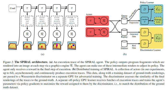
Note: no trajectories are omitted in the policy learner. Instead, the [math]\displaystyle{ D }[/math] updates is decoupled from the [math]\displaystyle{ \pi }[/math] updates by introducing a replay buffer that serves as a communication layer between the actors and the discriminator learner. That allows the latter to optimize [math]\displaystyle{ D }[/math] at a higher rate than the training of the policy network due to the difference in network sizes ([math]\displaystyle{ \pi }[/math] is a multi-step RNN, while [math]\displaystyle{ D }[/math] is a plain CNN). Even though sampling from a replay buffer inevitably results in smoothing of [math]\displaystyle{ p_{g} }[/math], this setup is found to work well in practice.
Experiments
Environments
Two rendering environment is introduced. For MNIST, OMNIGLOT and CELEBA generation an open-source painting librabry LIMBYPAINT (libmypaint contributors, 2018).) is used. The agent controls a brush and produces a sequence of (possibly disjoint) strokes on a canvas C. The state of the environment is comprised of the contents of [math]\displaystyle{ C }[/math] as well as the current brush location [math]\displaystyle{ l_{t} }[/math]. Each action [math]\displaystyle{ a_{t} }[/math] is a tuple of 8 discrete decisions [math]\displaystyle{ (a_t^1; a_t^2; ... ; a_t^8) }[/math] (see Figure 3). The first two components are the control point [math]\displaystyle{ p_{c} }[/math] and the endpoint [math]\displaystyle{ l_{t+1} }[/math] of the stroke.
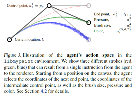
The next 5 components represent the appearance of the stroke: the pressure that the agent applies to the brush (10 levels), the brush size, and the stroke color characterized by a mixture of red, green and blue (20 bins for each color component). The last element of at is a binary flag specifying the type of action: the agent can choose either to produce a stroke or to jump right to [math]\displaystyle{ l_{t+1} }[/math].
In the MUJOCO SCENES experiment, we render images using a MuJoCo-based environment (Todorov et al., 2012). At each time step, the agent has to decide on the object type (4 options), its location on a 16 [math]\displaystyle{ \times }[/math] 16 grid, its size (3 options) and the color (3 color components with 4 bins each). The resulting tuple is sent to the environment, which adds an object to the scene according to the specification.
Datasets
MNIST
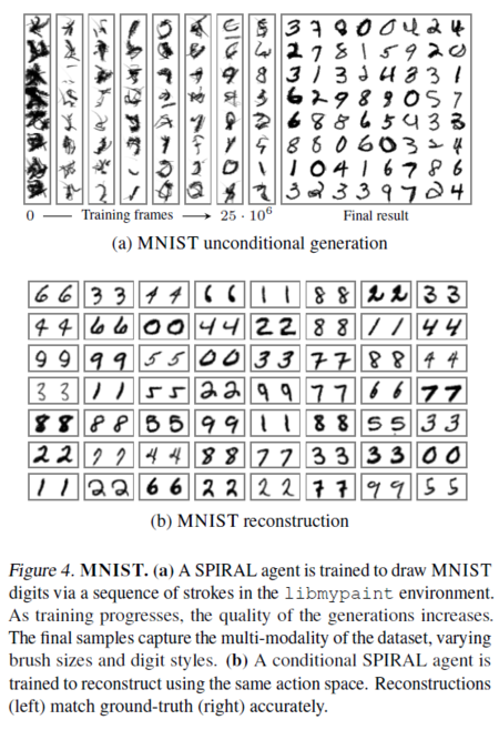
For the MNIST dataset, two sets of experiments are conducted:
1- In this experiment, an unconditional agent is trained to model the data distribution. Along with the reward provided by the discriminator, a small negative reward is provided to the agent for each continuous sequence of strokes to encourage the agent to draw a digit in a continuous motion of stroke. Example of such generation is depicted in the Fig 4a.
2- In the second experiment, an agent is trained to reproduce a given digit. Several examples of conditional generated digits are shown in Fig 4b.
OMNIGLOT
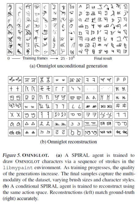
Now the trained agents are tested in a similar but more challenging setting of handwritten characters. As can be seen in Fig 5a, the unconditional generation has a lower quality compared to digits in the previous dataset. The conditional agents, on the other hand, were able to reach a convincing quality (Fig 5b). Moreover, as OMNIGLOT has lots of different symbols, the model that we created was able to learn a general idea of image production without memorizing the training data. We tested this result by inputting new unseen line drawings to our trained agent. As we concluded, it provided excellent results as shown in Figure 6.
For the MNIST dataset, two kinds of rewards, discriminator score and [math]\displaystyle{ l^{2}-\text{distance} }[/math] has been compared. Note that the discriminator based approach has a significantly lower training time and lower final [math]\displaystyle{ l^{2} }[/math] error.
Following (Sharma et al., 2017), also a “blind” version of the agent without feeding any intermediate canvas states as an input to [math]\displaystyle{ \pi }[/math] is trained. The training curve for this experiment is also reported in Fig 8a.
(dotted blue line) The results of training agents with discriminator based and [math]\displaystyle{ l^{2}-\text{distance} }[/math] approach is shown in Fig 8a as well.
CELEBA
Since the libmypaint environment is also capable of producing complex color paintings, this direction is explored by training a conditional agent on the CELEBA dataset. In this experiment, the agent does not receive any intermediate rewards. In addition to the reconstruction reward (either [math]\displaystyle{ l^2 }[/math] or discriminator-based), earth mover’s distance between the color histograms of the model’s output and [math]\displaystyle{ x_{target} }[/math] is penalized. (Figure 7)
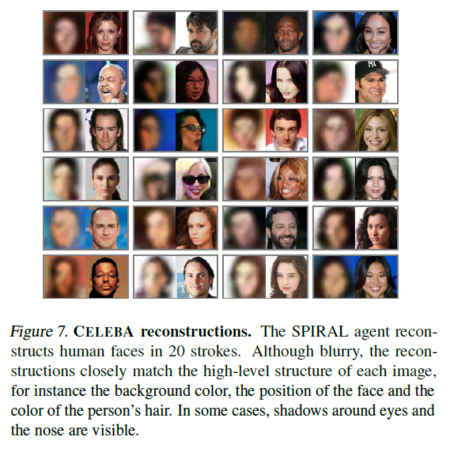
Although blurry, the model’s reconstruction closely matches the high-level structure of each image such as the background color, the position of the face, and the color of the person’s hair. In some cases, shadows around eyes and the nose is visible.
MUJOCO SCENES
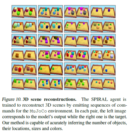
For the MUJOCO SCENES dataset, the trained agent is used to construct simple CAD programs that best explain input images. Here only the case of the conditional generation is considered. Like before, the reward function for the generator can be either the [math]\displaystyle{ l^2 }[/math] score or the discriminator output. In addition, there are not any auxiliary reward signals. This model has the capacity to infer and represent up to 20 objects and their attributes due to its unrolled 20 time steps.
As shown in Figure 8b, the agent trained to directly minimize [math]\displaystyle{ l^2 }[/math] is unable to solve the task and has significantly higher pixel-wise error. In comparison, the discriminator based variant solves the task and produces near-perfect reconstructions on a holdout set (Figure 10).
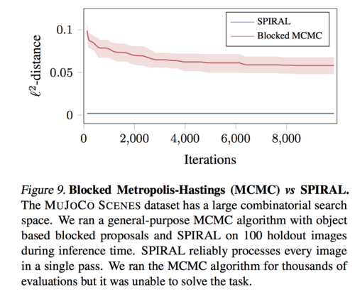
For this experiment, the total number of possible execution traces is [math]\displaystyle{ M^N }[/math], where [math]\displaystyle{ M = 4·16^2·3·4^3·3 }[/math] is the total number of attribute settings for a single object and N = 20 is the length of an episode. Then a general-purpose Metropolis-Hastings inference algorithm that samples an execution trace defining attributes for a maximum of 20 primitives was run on a set of 100 images. These attributes are considered as latent variables. During each time step of the inference, the attribute blocks (including presence/absence tags) corresponding to a single object are evenly flipped over the appropriate range. The resulting trace is presented as an output sample by the environment and then the output sample is accepted or rejected using the Metropolis-Hastings update rule, where the Gaussian likelihood is centered on the test image and the fixed diagonal covariance is 0.25. From Figure 9, the MCMC search baseline cannot solve the task even after a lot of evaluation.
Discussion
As in the OMNIGLOT experiment, the [math]\displaystyle{ l^2 }[/math]-based agent demonstrates some improvements over the random policy but gets stuck and as a result fails to learn sensible reconstructions (Figure 8b).
Scaling visual program synthesis to the real world and combinatorial
datasets has been a challenge. It has been shown that it is possible to train an adversarial generative agent employing
black-box rendering simulator. Our results indicate that
using the Wasserstein discriminator’s output as a reward
function with asynchronous reinforcement learning can provide
a scaling path for visual program synthesis. The current
exploration strategy used in the agent is entropy-based but
future work should address this limitation by employing sophisticated
search algorithms for policy improvement. For
instance, Monte Carlo Tree Search can be used, analogous
to AlphaGo Zero (Silver et al., 2017). General-purpose
inference algorithms could also be used for this purpose.
Critique and Future Work
- The architecture isn't new but it's a nice application and it's fun to watch the video of the robot painting in real life. SPIRAL's GAN-like idea continues the vein of connecting actor-critic RL with GANs like " reinforcement learning from human preferences" , Christiano et al 2017 or GAIL:
- Future work should explore different parameterizations of action spaces. For instance, the use of two arbitrary control points is perhaps not the best way to represent strokes, as it is hard to deal with straight lines. Actions could also directly parametrize 3D surfaces, planes, and learned texture models to invert richer visual scenes.
- A potential application can be in the field of medical images specifically to enhance and recolor histopathology slides for better detection. Also, image restoration problems could be addressed based on these approaches.
- On the reward side, using a joint image-action discriminator similar to BiGAN/ALI (Donahue et al., 2016; Dumoulin et al., 2016) (in this case, the policy can be viewed as an encoder, while the renderer becomes a decoder) could result in a more meaningful learning signal, since D will be forced to focus on the semantics of the image.
- The paper could also provide an avenue to further explore inverse simulation and program synthesis on applications ranging from vision , graphics, speech, music and scientific simulators.
- The paper provides a novel framework for designing and evaluating generative approaches for drawing and painting without explicit supervision. However, more research might be required to design a proper reward function for each specific domain. For some applications can be beneficial to let the actor explore a wider number of alternatives without applying a penalization for using more drawing movements. In other words, by leaving the actor work in a wider search space, some sort of creativity could emerge and newer or better procedures might be discovered.
Other Resources
- Code implementation [3]
References
- Yaroslav Ganin, Tejas Kulkarni, Igor Babuschkin, S.M. Ali Eslami, Oriol Vinyals, [[4]].